The Normal Distribution
420 likes | 515 Vues
Learn about continuous random variables, normal distributions, and empirical rules for data analysis with clear examples and concepts. Explore how to find proportions, percentiles, and relative positions in statistical data.

The Normal Distribution
E N D
Presentation Transcript
The Normal Distribution Chapter 2
Continuous Random Variable • A continuous random variable: • Represented by a function/graph. • Area under the curve represents the proportions of the observations • Total area is exactly 1. • How do we locate the median for a continuous random variable? the mean? • The median is the value that divides the graph into equal area while the mean is the “balance” point.
Continuous Random Variable 1 A= .4(1) =0.4 0.4 0.5 What percent of the observations lie below 0.4? 40%
Continuous Random Variable 2 A= 1.4(.5) =0.7 0.6 What proportion of the observations lie above 0.6? Notice, to find proportion for observation above, we can use the complement rule.
Continuous Random Variable 3 • Where is the mean and median? • How will the curve change as s changes?
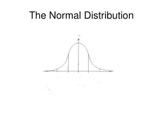
Normal Distributions • Symmetric, single-peaked, and mound-shaped distributions are called normal distributions • Normal curves: • Mean = median • The mean m and standard deviation s completely determine the shape
The Normal Curve • Will finding proportions work different than previous random variable examples? • Empirical Rule Discovery
68-95-99.7 Rule Applet
68-95-99.7 Rule 34% 34% .15% 2.35% 13.5% 13.5% 2.35% Applet
Percentiles? 16th 50th 84th 34% 34% 2.35% 13.5% 13.5% 2.35%
What’s Normal in Statistics? • Normal distributions are good descriptions for real data allowing measures of relative position to be easily calculated (i.e. percentiles) • Much of statistical inference (in this course) procedures area based on normal distributions • FYI: many distributions aren’t normal
Distribution of dates is approximately normal with mean 1243 and standard deviation of 36 years. 1135 1171 1207 1243 1279 1315 1351
Assume the heights of college women are normally distributed with a mean of 65 inches and standard deviation of 2.5 inches. 57.5 60 62.5 65 67.5 70 72.5
What percentage of women are taller than 65 in.? 50% 57.5 60 62.5 65 67.5 70 72.5
What percentage of women are shorter than 65 in.? 50% 57.5 60 62.5 65 67.5 70 72.5
What percentage of women are between 62.5 in. and 67.5 in.? 68% 57.5 60 62.5 65 67.5 70 72.5
What percentage of women are between 60 in. and 70 in.? 95% 57.5 60 62.5 65 67.5 70 72.5
What percentage of women are between 60 and 67.5 in? 68% 13.5% 81.5% 57.5 60 62.5 65 67.5 70 72.5
What percentage of women are shorter than 70 in.? 50% 34% 13.5% 97.5% 57.5 60 62.5 65 67.5 70 72.5
Iliana’s Grade • After 5 weeks of class Iliana must transfer from a stat class at Lanier to this class. Last week was the chapter 1 test in both classes. Iliana scored a 61 out of 70. Let’s say our test was out of 100 points. What score should she be given?
Iliana’s claim • Iliana claims that her test at Lanier was harder than our test. • Does your previous method of assigning a grade take in consideration difficulty? • If we have all of the data, what important facts can we utilize to improve our assignment of Iliana’s grade?
Important Facts • Maximum possible on our test was 100 pts while Lanier’s test was 70 pts. • Mean score on Lanier’s test was 50.5 pts while our test was 77.2 pts. • Standard deviation on Lanier’s test was 5.3 pts while ours was 8.1 pts. • Test scores from both high schools tend to be normally distributed. • How will we fairly assign Iliana’s score?
Iliana Lanier’s distribution 50.5 55.8 61.1 66.4
Iliana Iliana 50.5 55.8 61.1 66.4 77.2 85.3 93.4 101.5 Lanier’s and McCallum’s distributions – class average Iliana’s score standard deviation • How can we find Iliana’s relative position?
Iliana’s score – class average standard deviation Formula • What is the formula to find the relative position for any distribution? z–score=
1. Suppose as student has taken two quizzes in a statistics course. On the first quiz the mean score was 32, the standard deviation was 8, and the student received a 44. The student obtained a 28 on the second quiz, for which the mean was 23 and the standard deviation was 3. If test scores are approximately normal, on which quiz did the student perform better relative to the rest of the class? First quiz: Second quiz:
3. A married couple is employed by the same company. The husband works in a department for which the mean hourly rate is $12.80 and the standard deviation is $1.20. His wife is employed in a department where the mean rate is $13.50 and the standard deviation is $1.80. Relative to their departments, which is better paid if the husband earns $14.60 and the wife earns $15.75? Husband: Wife:
What percent of employees in the wife’s department earn better than her?
What would the wife need to earn to match her husband’s relative position? Husband: Wife: The wife would need to earn $16.20 to match the husband’s relative position.
If the husband wanted to earn in the 95th percentile, how much should he earn per hour? Need a z-score of 1.65!
The husband will need to earn at least $14.78 to be in the 95th percentile.
– 2 2
5.5% 94.5% 89% 44.5% z-score = –1.60 z-score = 1.60 The middle 89% of the data ranges from 18.81 to 55.03 ppb.
Warm Up Answer Check • Probability of a president being 52 year old or younger is .3192. • Probability of SAT math score less than 540 is .8907. • Probability of Aprils having one or fewer frost days is .2389. • Probability of hotdogs having over 500 mg of sodium is .2177.
PREZ Data is approximately normal.
SATM Data is fairly normal.
FROST Data is not normal.
HOTDG Data is approximately normal.
