Download
1 / 8
80 likes | 264 Vues
Sea State Bias in Satellite Radar Altimetry - Revisited. Jessica Hausman and Victor Zlotnicki. Sea State Bias. Jason-1. Actual sea surface. ~ 3% of SWH. Measured sea surface. x. Solve for SSB SSH 2 – SSH 1 = (SSB 2 – SSB 1 ) + E

E N D
Sea State Bias in Satellite Radar Altimetry - Revisited Jessica Hausman and Victor Zlotnicki
Sea State Bias Jason-1 Actual sea surface ~ 3% of SWH Measured sea surface x
Solve for SSB SSH2 – SSH1 = (SSB2 – SSB1) + E • 1 and 2 indicate time at the same geographical location. • SSH is the sea surface height above the ellipsoid • E is an error term (Gaspar et al. 2002). • Typically t1 is a time mean encompassing several years. • This technique may not resolve all of the physics that occur in the ocean, which can “leak” into the SSB calculation.
To investigate we calculate SSB using SWH (significant wave height) and U (wind speed) from Jason-1 2003-2004 and SSH from ECCO2 and Labroue et al 2004. • Compute SSB by using a time difference subtracted from a time mean (Direct) and from collinear consecutive cycle differences (CCD). • The CCD method has a much shorter time difference (~10 days, the time difference between cycles) and any oceanic signals should be resolved with this method.
2003-2004 SWH(J1) vs. SSH(ECCO2) Correlation CCD, ∆SWH vs ∆SSH Direct, SWH vs SSH-<SSH>
ECCO2 CCD : SSB=SWH(9x10⁻⁴ – 1x10⁻⁴SWH – 1x10⁻⁵U + 2x10⁻⁷U2) Parametric, SSB = SWH( + SWH+U + U2) Labroue CCD: SSB=SWH(-5x10⁻² + 3x10⁻³SWH – 2x10⁻³U + 6x10⁵U2) mm mm U m/s U m/s ECCO2 Direct: SSB=SWH(2x10⁻³ – 3x10⁻⁴SWH – 2x10⁻⁴U + 8x10⁻⁶U2) Labroue Direct: SSB=SWH(3x10⁻² – 4x10³SWH – 3x10⁻³U + 1x10⁻⁴U2) mm mm U m/s U m/s
ECCO2, CCD Labroue, CCD Nonparametric,SSB = SSHin(x1j, x2i) + SSB(x1i) n(x1j, x2i), mean=-0.78 mm, std=53 mm mean=-136 mm, std=49 mm mm mm ECCO2, Direct Labroue, Direct mean=0.82 mm, std=74 mm mean=3 mm, std=40 mm mm mm
Conclusions • Parametric shows that CCD gives values closest to those expected • Labroue nonparametric CCD gives values closer to expected than Direct • ECCO nonparametric does not show much difference between CCD and Direct because of the small scales