Download
1 / 23
250 likes | 300 Vues
Enhance land cover classification accuracy using geostatistical techniques on images affected by spatially correlated noise and smoke, with applications for fire-affected areas. Explore methods, models, and examples to improve classification performance.

E N D
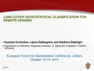
LAND COVER GEOSTATISTICAL CLASSIFICATION FOR REMOTE SENSING • KęstutisDučinskas, Lijana Stabingiene and Giedrius Stabingis • Department of Statistics, Klaipeda University, H. Manto 84, Klaipeda LT-92294, Lithuania European Forum for Geostatistics Conference, Lisbon, October 12-14 ,2011
Relevance and the main objective • Problem - non geostatistical classification methods are not efficient when territory is covered by the smoke of fire. • Objective – to increase accuracy of land cover classification from remotely sensed imagery • Proposed geostatistical classification technique is realised in the examples with images corrupted by spatially correlated Gaussian noise. Territory is covered with the spatially correlated smoke. Image from NASA MODIS satellite.
Introduction 1 • Switzer [1] was the first to treat classification of spatial data. • For features based on Gaussian Markov model, the influence of texture rotation to image classification is considered by Deng and Clausi [2]. • Spatial contextual classification problems arising in geospatial domain is considered by Shekhar [3]. • Atkinson, Naser [4], [5] incorporated geostatistical information of features into plug-in versions of classifiers based on the marginal distribution of the observation to be classified.
Introduction 2 • Image classification problem is to divide an observed image into several homogeneous regions by labeling pixels, based on feature information and on information about spatial adjacency relationships with training sample. • The stationary Gaussian Random Field (GRF) model for features and MRF model for class labels are considered. • In the case of partial parametric uncertainty, the plug-in BDF is proposed. • This is the generalization of the discriminant function derived in the case of training sample with fixed training sample and fixed prior probabilities for labels [6].
Introduction 3 • Geostatistical techniques that utilise spatial information in classification can be split into two distinct groups.(Atkinson,2000) • In the first, spatial information is used to provide data on texture. It is implicit in such approaches that texture varies spatially across the image, and particularly between the classes of interest, so that data on texture can be used to inform classification (pixel-by pixel classification) . • In the second group, spatial information is used to smooth the classified image. The rationale for smoothing is that inaccuracies that arise from simple spectral classification applied on a pixel-by-pixel basis can be reduced using the spatial dependence between neighbouring pixels. Proximate pixels are likely to be similar and this dependence can be formalised and utilised to increase classification accuracy. The goal is to choose a smoothing function based upon this spatial dependence.
Methods 1 • The marginal model of the observation Z(s) in class is the error term is generated by zero-mean stationary GRF with covariance function: , , - spatial correlation function, , - scale parameter. - label set, - set of training pixels.
Methods 2 - training sample. - labels vector. - features vector Assume that the Z model for given Y=y is Assumption. The conditional distribution of Y(s0) given T=t depends only on Y=y, i.e.
Methods 3 Dependent BDF classification BDF for the classification of Z0 given T=t (with Z=z, Y=y) under the Assumption is: . where .
Methods 3 If Z0 is assumed to be independent to T, then BDF (BDFI) is implemented by Atkinson(2004,2010). It has a following form
Methods 4 Bayes error rate for BDF . . Bayes error rate for BDFI . .
Methods 4 PBDF to the classification problem based on BDF PBDFI to the classification problem based on BDFI (If Z0 is assumed to be independent to T)
Methods 5 The actual error rate for PBDF where
Methods 5 The actual error rate for PBDFI
Land cover classification example • The example of land cover classification from remotely sensed image into two classes (Woodland:black; Grassland:white). • Additive stationary GRF with isotropic exponential covariance is applied to the image. • Such situation can occur during fire or fog. • Our proposed classification methods, using different PBDF and PBDFI are applied.
Land cover classification example • N0=NN(16) neighborhood model is used. • Supervised classification methods are compared with unsupervised classification method using co-occurrence matrices (GLCM) by using the empirical error rates.
Forest territory classification example Real satellite image crop Image with spatially correlated GRF Training sample
Classification results of real image Classification with PBDF Classification with PBDFI Classification with GLCM average The empirically calculated errors.
Conclusions • The results of performed calculations give us the strong argument to encourage the users do notignore the spatial dependence in image classification and reconstruction. • The advantage of BDF against BDFI and the advantage of PBDF against PBDFI are shown numerically and visually in image restoration and in remotely sensed image classification examples.
References • [1] Switzer P. Extensions of linear discriminant analysis for statistical classification of remotely sensed satellite imagery. Math. Geol 1980; 12:367–376. • [2] Deng H, Clausi DA. Gaussian MRF rotation invariant features for image classification. IEEE Trans Pattern Anal Machine Intell 2004; 26(7):951-955. • [3] Shekhar S, Schrater PR, Vatsavai RR, Wu W, Chawla S. Spatial contextual classification and prediction models for mining geospatial data. IEEE Trans on Multimedia 2002; 4(2):174-188. • [4] Atkinson, P. M. (2004). Spatially weighted supervised classification for remote sensing. International journal of applied earth observation and geoinformation, 5 , 277–291. • [5] Atkinson, P. M., & Naser, D. K. (2010). A geostatistically weighted k-nn classifier for remotely sensed imagery. Geographical analysis, 42 , 204–225. • [6] Dučinskas K. Approximation of the expected error rate in classificattion of the gaussian random field observations. Statistics and Probability Letters 2009, 79:138–144.