Linear Programming
Department of Business Administration. FALL 200 7 -0 8. Linear Programming. by Asst. Prof. Sami Fethi. Linear Programming.

Linear Programming
E N D
Presentation Transcript
Department of Business Administration FALL 2007-08 Linear Programming by Asst. Prof. Sami Fethi
Linear Programming • Linear Programming: is a mathematical technique for solving constrained maximization and minimization problems when there is more than one constraint and both the objective function to be optimized and constraints faced are linear. • Assumes that the Objective Function is Linear • Assumes that All Constraints Are Linear
Linear Programming • A basic assumption of linear programming is that commodities can be produced with only a limited number of input combinations. Or the objective function that the organisation seeks to optimise (i.e. maximize or minimize) as well as the constraints that it faces, are linear and can be represented graphically by straight lines. This means that we assume that input and output prices are constant and that we have CRS.
Applications of Linear Programming • Optimal Process Selection: Given input prices and the quantity of the commodity that the firm wants to produce, linear programming can be used to determine the optimal combination of processes needed to produce the desired level and output at the lowest possible cost, subject to labor, capital and the other constraints that the firm may face.
Applications of Linear Programming • Optimal Product Mix: Usually most firms produce a variety of products rather than a single one and must determine how to best use their plants, labor, and other inputs to produce the combination or mix of products that maximizes their total profits subject to the constraints they face i.e., the production of a particular commodity may lead to the highest profit per unit but may not use all the firm’s resources. The unused resources can be used to produce another commodity, however this product mix may not lead to overall profit maximization for the firm as a whole.
Applications of Linear Programming • Satisfying Minimum Product Requirements: production often requires that certain minimum product requirements be met at minimum cost. i.e., the manager of a college dinning hall may be required to prepare meals that satisfy the minimum daily requirements of protein, minerals, and vitamins at a minimum cost. Due to the various nutrients and different prices, this problem can be complex and solved easily by linear programming by specifying the total cost function that manager seeks to minimize and the various constraints that he or she must meet or satisfy.
Applications of Linear Programming • Long-Run Capacity Planning: An important question that firms seek to answer is how much contribution to profit each unit of the various inputs makes. If this exceeds the price that the firm must pay for the input, this is an indication that the firm’s total profit would increase by hiring more of the input. If the input is underused, this means that some units of the input need not be hired or can be sold to other firms without affecting the firm’s output. This can be very useful to the firm in its investment decisions and future profitability while determining the marginal contribution of an input.
Applications of Linear Programming • Least Cost Shipping Route: Linear programming has also been applied to determine the least cost route for shipping commodities from plants in different locations to warehouses in other locations and from there to different markets ( so called Transportation Problems).
Applications of Linear Programming • Airline Operations Planning • Output Planning with Resource and Process Capacity Constraints • Distribution of Advertising Budget • Routing of Long-Distance Phone Calls • Investment Portfolio Selection • Allocation of Personnel Among Activities
Production Processes A basic assumption of linear programming is that commodities can be produced with only a limited number of input combinations. With two inputs, capital, and labour each input combination, or capital labour ratio, is called production process and can be represented by a straight line ray from the origin in input space. Production processes are graphed as linear rays from the origin in input space. Production isoquants are line segments that join points of equal output on the production process rays.
Left panel Figure shows that a particular commodity can be produced with three processes. Process 1 with K/L=2, process 2 with K/L=1, and process 3 with K/L=1/2. Each of these processes is represented by the ray from the origin with slope equal to the particular K/L ratio used. These process can be used by a firm to produce a particular commodity. Joining these points, we get the isoquants for 100Q and 200Q. Twice as many input provides twice as much output. i.e., CRS Production Processes Processes Isoquants
If the firm faced only one constraint, such as isocost line GH in the left panel, the feasible region, or the area of attainable input combinations, is represented by shaded triangle OJN. The firm can purchase any combination of labor and capital on or below isocost line GH. The best or optimal solution is at point E. The right panel shows that the firm faces no cost constraint, but the feasible region is shaded area ORST and the optimal solution is at point S. Production Processes Feasible Region Optimal Solution (S)
Formulating and Solving Linear Programming Problems • Express Objective Function as an Equation and Constraints as Inequalities • Graph the Inequality Constraints and Define the Feasible Region • Graph the Objective Function as a Series of Isoprofit or Isocost Lines • Identify the Optimal Solution
Profit Maximization-Example Maximize Subject to (objective function) (input A constraint) (input B constraint) (input C constraint) (non-negativity constraint) = $30QX + $40QY 1QX + 1QY 7 0.5QX + 1QY 5 0.5QY 2 QX, QY 0
Profit Maximization-Extreme Points-Simplexmethod Multiple Optimal Solutions New objective function has the same slopeas the feasible region at the optimum If we have the new isoprofit line H’J’, the value of profit = $ 240. This is because all product mixes along EF gives the same profit value. i.e., at point M (3X, 3.5Y), we get the same profit such as $240= $24(3)+ $48(3.5).
Profit Maximization- Algebraic Solution Algebraic Solution Points of Intersection Between Constraintsare Calculated to Determine the Feasible Region
Profit Maximization Algebraic Solution Profit at each point of intersection between constraintsis calculated to determine the optimal point (E) i.e., at point E =$240 = $30(QX=4) + $40(QY=3)
Cost Minimization-Example Minimize Subject to C = $2QX + $3QY 1QX + 2QY 14 1QX + 1QY 10 1QX + 0.5QY 6 QX, QY 0 (objective function) (protein constraint) (minerals constraint) (vitamins constraint) (nonnegativity constraint)
Cost Minimization Feasible Region Optimal Solution (E)
Cost Minimization Algebraic Solution Cost at each point of intersection between constraintsis calculated to determine the optimal point (E) The manager minimizes costs by using 6 units of food X and 4 units of food Y at point E at a cost of C = $2(6)+ $3(4)=$24.
The Dual Problem and Shadow prices • Every linear programming problem, called the primal problem, has a corresponding or symmetrical problem called the dual problem. A profit-maximization primal problem has a cost-minimization dual problem, and vice versa. The solution of a dual problem yields the shadow prices. They give the change in the value of the objective function per unit change in each constraint in the primal problem. According to the duality theorem, the optimal value of the objective function is the same in the primal and in the corresponding dual problems.
Dual of the Profit Maximization Problem Maximize Subject to = $30QX + $40QY 1QX + 1QY 7 0.5QX + 1QY 5 0.5QY 2 QX, QY 0 (objective function) (input A constraint) (input B constraint) (input C constraint) (nonnegativity constraint) Minimize Subject to C = 7VA + 5VB + 2VC 1VA + 0.5VB $30 1VA + 1VB + 0.5VC $40 VA, VB, VC 0
Dual of the Profit Maximization Problem • In the dual problem we seek to minimize the shadow prices of inputs A, B, and C used by the firm. Defining VA, VB, as the shadow prices of inputs and C as the total imputed values of the fixed quantities of inputs available to the firm, we can write the dual objective function as minimizeC=7 VA+5 VB+2 VC • Thus the constraints of the dual problem can be written as follow: 1VA + 0.5VB $30 1VA + 1VB + 0.5VC $40 so VC=0 due to slack variable. 1VA + 0.5VB= $30 1VA + 1VB = $40 therefore 0.5VB=$10, VB=$20 and VA=$20 C=7 ($20)+5 ($20) +2 (0)=$240 this is the minimum cost.
Dual of the Cost Minimization Problem Minimize Subject to C = $2QX + $3QY 1QX + 2QY 14 1QX + 1QY 10 1QX + 0.5QY 6 QX, QY 0 (objective function) (protein constraint) (minerals constraint) (vitamins constraint) (nonnegativity constraint) Maximize Subject to = 14VP + 10VM + 6VV 1VP + 1VM+ 1VV $2 2VP + 1VM + 0.5VV $3 VP, VM, VV 0
Dual of the Cost Minimization Problem • Since we know that from the solution of the primal problem that vitamin constraint is a slack variable, so that VV=0, subtracting the first from the second constraint, we can get the solution of the dual problem as follow: 2VP + 1VM =3 1VP + 1VM= 2 , therefore VP =$1 and VM =$1 The profit as follows: = 14($1)+ 10($1)+ 6($0) = $24.
The End Thanks

