Download
1 / 13
130 likes | 180 Vues
“Better” Covariance Matrix Estimation for Markowitz Port Opt. Rez, Nathan, Ka Ki, Dzung, Pryianka. This Week. 1. Implemented Industry Factors Estimator 2. Readjusted Ledoit Constraint to handle monthly returns computations. Leads to more closely matching results.

E N D
“Better” Covariance Matrix Estimation for Markowitz Port Opt. Rez, Nathan, Ka Ki, Dzung, Pryianka
This Week • 1. Implemented Industry Factors Estimator 2. Readjusted Ledoit Constraint to handle monthly returns computations. Leads to more closely matching results. 3. Implemented option to calculate returns without dividends. • 4. Implemented “not-looking-into-future” • 5. Ran the software for a NEW data set - 2006 to 2009 (out of sample window)
Industry Factors Estimator • So you were right - we needed two Betas - one for the market and one for the industry sector. - used linear least square matrix version to get these two Betas…
Results • Ledoit and Wolf standard deviation • = 10.84 • Our standard deviation = 9.34 • Our portfolio return value = not yet computed
Ledoit constraint improvement • We have implemented the formula to convert the expected returns constraint from annual to monthly since all our computations are done on a monthly basis… • Now the constrained numbers match more closely.. • Qannual = 0.2 Qmonthly = 0.0154
not-looking-into-the-future|constrained – unconstrained| In general, the differences match pretty closely. So that’s good…
Moral of the story • Our values are generally lower. WHY? • Yes intuitively it should be higher, BUT • Consider this possible factor: • 1. CRSP cleaned up the data • Our number of stocks differ for each given year • Our number of stocks is sometimes significantly GREATER • Specific number for example.. Ledoit lowest year 909 stocks, highest year 1314 • Specific number for example… US lowest year 1183 • Stocks, highest year 1379 • Our average = 1273. • So since our N is somewhat HIGHER on average, and the investment is distributed across a greater number of (i.i.d?) stocks, it is perhaps reasonable that our risk values are lower… based on what we learned in class? Lec 1 or 2… Assuming that model holds to an extent…
“The Future”: Portfolio Performances (Unconstrained) 2006 – 2009 (The Lehman Brother Years…)
Returns without dividends • Why? Well the returns look more reasonable now… • Specifically, the return for • Identity model: 10 to 11 percent… • With dividends last presentation: 14% • We would like to note that neither of the authors we are studying published their returns results… hmmmmmmm
Future Plans • If we have time we could implement an estimator where stocks with positive betas are in one block, and stocks with negative betas are in the other block. We can probably leverage the market model code for this… • Why? Benninga thought this might be more “financially oriented” (pg. 30, Jan 2006, Ben. Paper…)
The End • Questions? • THANKS!