Introduction to Radar Systems
Introduction to Radar Systems. Chris Allen (callen@eecs.ku.edu) Course website URL people.eecs.ku.edu/~callen/725/EECS725.htm. Outline. Syllabus Instructor information, course description, prerequisites Textbook, reference books, grading, course outline Preliminary schedule Introductions

Introduction to Radar Systems
E N D
Presentation Transcript
Introduction to Radar Systems • Chris Allen (callen@eecs.ku.edu) • Course website URL people.eecs.ku.edu/~callen/725/EECS725.htm
Outline • Syllabus • Instructor information, course description, prerequisites • Textbook, reference books, grading, course outline • Preliminary schedule • Introductions • What to expect • First assignment • Radar fundamentals • Active RF/microwave remote sensing • Electromagnetic issues • Antennas • Resolution (spatial, range)
Syllabus • Prof. Chris Allen • Ph.D. in Electrical Engineering from KU 1984 • 10 years industry experience Sandia National Labs, Albuquerque, NM AlliedSignal, Kansas City Plant, Kansas City, MO • Phone: 785-864-8801 • Email: callen@eecs.ku.edu • Office: 3024 Eaton Hall • Office hours: Monday through Friday, 11 am to noon • Course description • Basic radar principles and applications. Radar range equation. Pulsed and CW modes of operation for detection, ranging, and extracting Doppler information.
Syllabus • Prerequisites • Signal analysis course (EECS 360) Fourier analysis, linear system analysis, MATLAB • Electromagnetics course (EECS 420) propagation, transmission lines, antennas • Probability and statistics course (EECS 461) functions of random variables • Introductory course on radio systems (EECS 622) (recommended)transmitter and receiver design, signal detection with noise • Textbook • Principles of Modern Radar: Basic Principles • by M.A. Richards, J.A. Scheer, W.A. Holm • SciTech Publishing, 2010, ISBN 1891121529
Syllabus • Reference books • Microwave Remote Sensing: Active and Passive – Vol. I by F. Ulaby, R. Moore, and A. FungArtech House, 1981, ISBN 0890061904 • Microwave Remote Sensing: Active and Passive – Vol. II by F. Ulaby, R. Moore, and A. FungArtech House, 1982, ISBN 0890061912 • Introduction to Airborne Radar, Second Editionby G. StimsonSciTech Publishing, 1998, ISBN 1891121014 • Introduction to Radar Systemsby M. SkolnikMcGraw-Hill , 2002, ISBN 0072881380
Syllabus • Reference books • Radio Frequency Principles and Applications by A. SmithIEEE Press, 1998, ISBN 0780334310 • Radar Principles for the Non-Specialistby J. Toomay and P. Hannen SciTech Publishing, 2004, ISBN 1891121340 • Radar: principles, technologies, applicationsby B. EddePrentice Hall, 1995, ISBN 0137523467 • Fundamentals of Radar Signal Processingby M. RichardsMcGraw-Hill, 2005, ISBN 0071444742
Grades and course policies • The following factors will be used to arrive at the final course grade: • Homework & quizzes 15 % Design project 15 % Midterm exam 35 % Final exam 35 % • Grades will be assigned to the following scale: • A 90 - 100 % B 80 - 89 % C 70 - 79 % D 60 - 69 % F < 60 % • These are guaranteed maximum scales and may be revised downward at the instructor's discretion. • Read the policies regarding homework, exams, ethics, and plagiarism.
Outline and schedule • Course Outline (subject to change) • Radar fundamentals system overview and signal properties(block diagram, radar frequencies, antennas, radar equation, accuracy and resolution) • Radar design issues(signal-to-noise ratio, sampling criterion, coherence) • Signal processing and detection(analog-to-digital conversion, coherent and incoherent processing) • Waveforms(pulse compression, sidelobes) • Remote sensing radars(altimeters, scatterometers, sidelooking radar, synthetic-aperture radar) • Ground-penetrating radar; Bistatic and multistatic radar; and more • Class Meeting Schedule • January: 22, 24, 27, 29, 31 • February: 3, 5, 7, 10, 12, 14, 17, 19, (no class on the 21st Eng Expo), 24, 26, 28 • March: 3, 8, 7, 10, 12, 14, (no class on the 17th, 19th, 21st Spring Break), 24, 26, 28, 31 • April: 2, 4, 7, 9, 11, 14, 16, 18, 21, 23, 25, 28, 30 • May: 2, 5, 7 • Final exam scheduled for Tuesday, May 13, 1:30 to 4:00 p.m.
Course website • URL: people.eecs.ku.edu/~callen/725/EECS725.htm • Contains – • Syllabus • Class assignments • Some supplemental course material • Project information (when issued) • Powerpoint files used in class presentations • continually updated to correct errors or enhanced • file contents typically span many presentations (class sessions) • max slide count ~ 100 • Links to recorded presentations (audio and Powerpoint) • Special announcements (when issued)
Introductions • Name • Major • Specialty • What you hope to get from of this experience • (Not asking what grade you are aiming for )
What to expect • Course is being webcast, therefore … • Most presentation material will be in PowerPoint format • Presentations will be recorded and archived (for duration of semester) • Not 100% reliable (occasionally recordings fail due to a variety of causes) • Student interaction is encouraged • Students may need to activate microphone before speaking • Homework assignments will be posted on website • Electronic homework submission logistics to be worked out • We may have guest lecturers later in the semester • To break the monotony, we’ll take a couple of 2-minute breaks during each class session (roughly every 15 to 20 min)
Your first assignment • Send me an email (from the account you check most often) • To: callen@eecs.ku.edu • Subject line: Your name – EECS 725 • Tell me a little about yourself and what knowledge you hope to gain from this experience
Background • Radar – radio detection and ranging • Developed in the early 1900s (pre-World War II) • 1904 Europeans demonstrated use for detecting ships in fog • 1922 U.S. Navy Research Laboratory (NRL) detected wooden ship on Potomac River • 1930 NRL engineers detected an aircraft with simple radar system • World War II accelerated radar’s development • Radar had a significant impact militarily • Called “The Invention That Changed The World” in two books by Robert Buderi • Radar’s has deep military roots • It continues to be important militarily • Growing number of civil applications • Objects often called ‘targets’ even civil applications
Variety of radar applications (examples) • Type Civil Military • Ground-based, stationary weather radar air defense monostatic radar astronomy missile defense traffic control perimeter defense • inverse SAR • Ground-based, stationary radar astronomy air defense (fence) multistatic missile defense • Ground-probing radar archeology tunnel detection ice sounding land-mine detection • Airborne/spaceborne collision avoidance search & track monostatic altimeter fuzing imaging (SAR) imaging/targeting scatterometer navigation • Airborne/spaceborne interferometric SAR covert radar multistatic planetary exploration • Tx: transmitter, Rx: receiver, Monostatic: co-located Tx & Rx;Bistatic: One Tx, one Rx, separated, Multistatic: multiple Tx or Rx, separated
Example fence radar: BMEWS • BMEWS: Ballistic Missile Early Warning System
Example weather radar: NEXRAD • NEXRAD Radar (WSR-88D) • ParametersS-band (2.7 to 3 GHz)PTX = 750 kW • Antennaparabolic reflector diameter: 8.5 mbeamwidth: 16.6 mrad (0.95°) • Rain off the coast of Brownsville, Texas
Example ground-penetrating radar • Mapping unmarked colonial era graves • Mapping agricultural drainage pipes
Characteristics of radar • Uses electromagnetic (EM) waves • Frequencies in the MHz, GHz, THz • Governed by Maxwell’s equations • Propagates at the speed of light • Antennas or optics used to launch/receive waves • Related technologies use acoustic waves • Ultrasound, seismics, sonar • Microphones, accelerometers, hydrophones used as transducers • Active sensor • Provides its own illumination • Involves both a transmitter and a receiver • Related technologies are purely passive • Radio astronomy, radiometers
Concepts and technologies used in radar • Radars are systems involving a wide range of technologies and concepts • An understanding of radar requires knowledge over this broad range of technologies and concepts • As new technologies emerge and new concepts are developed, radar capabilities can grow and improve • New enabling technologies signify breakthroughs
Concepts and technologies used in radar • Electromagnetics • Antennas (multiple roles) • Impedance transformation (free-space intrinsic impedance to transmission-line characteristic impedance) • Propagation mode adapter (free-space fields to guided waves) • Spatial filter (radiation pattern – direction-dependent sensitivity) • Polarization filter (polarization-dependent sensitivity) • Phase center • Arrays • Calibration targets (enhanced radar cross section RCS) • Passive (trihedral, sphere, Luneberg lens) • Active • Coded (time, amplitude, frequency, phase, polarization) • RCS suppression (stealth) • Reflection, refraction, diffraction, propagation, absorption, dispersion
Concepts and technologies used in radar • Electromagnetics • Scattering • Objects (shape, composition, orientation) • Surface (specular, facets, Bragg resonance, Kirchhoff scattering, small-perturbation) • Volume (Rayleigh, Mie) • Materials (permittivity, permeability, conductivity) • Absorber • Radome • Doppler shift • Coherence and interference • Fading • Fresnel zones • Numerical modeling, simulation, inversion • Finite difference time domain (FDTD) • Commercial CAD tools (HFSS, CST) • EM compatibility (emission, conduction, interference, susceptibility)
Concepts and technologies used in radar • RF/microwave • Oscillators (stable reference) • Phase-locked loops (PLLs) • Frequency synthesizers • Frequency multipliers • Filters (SAW, lumped element, distributed) • Amplifiers (low noise, small signal, power) • Mixers (double balanced, single-sideband) • Limiters / switches / detectors
Concepts and technologies used in radar • Digital • Timing and control • Pulse repetition frequency (PRF) • Switch control signals • Interpulse coding • Waveform sequencing • Waveform generation • D/A converters • Direct digital synthesizer (DDS) • Arbitrary waveform generator (AWG) • I/Q modulation • Data acquisition • A/D converters • Data buffering • Real-time processing • Data storage
Concepts and technologies used in radar • Math • System geometry (monostatic, bistatic, multistatic) • Sampling theory • Aliasing and ambiguities (range, Doppler, spatial, phase) • Oversampling (integration, decimation) • Undersampling • Signal analysis (correlation, convolution, spectral analysis) • Waveforms / Coding theory • Pulsed • Unmodulated • Phase codes (binary, polyphase, quadrature, complementary) • Linear FM (chirp) • Window functions • Continuous wave (CW) • Unmodulated • Stepped FM • Linear FM • Noise
Concepts and technologies used in radar • Signal processing • Fourier analysis • Cross-correlation / cross-covariance • FIR and IIR filters (low pass, band pass, high pass, notch, all pass) • Matched filters • Pulse compression • Along-track focusing • Phase coherence • Detection and estimation (noise, interference, clutter) • Fast time / slow time / spatial domains • Coherent / incoherent integration • Synthetic aperture / interferometry / tomography • Motion compensation
Concepts and technologies used in radar • Auxiliary sensors • Inertial navigation system (INS) • Accelerometers • Gyroscopes • Global positioning satellite (GPS) • Knowledge of position & velocity • Pulse per second (PPS) reference • Differential GPS for decimeter precision
Radar measurement capabilities • Presence of target (detection ) • Range (distance and direction) • Received signal strength • Radial velocity (Doppler frequency shift) • Spatial distribution (mapping) • Various target characteristics • Particle size distribution (e.g., precipitation) • Surface roughness • Water content (e.g., soil, snow) • Motion characteristics (e.g., aircraft engine rotation rate, breathing) • Surface displacement (e.g., subsidence)
Airborne SAR block diagram • New terminology:SAR (synthetic-aperture radar)Magnitude imagesMagnitude and Phase ImagesPhase HistoriesMotion compensation (MoComp)Autofocus • AutofocusTiming and ControlInertial measurement unit (IMU)GimbalChirp (Linear FM waveform)Digital-Waveform Synthesizer
Introduction via a simple radar • Block diagram shows the major subassemblies in a simple radar system.
Simple radar • R • CNTL • RF • Begin with the frequency synthesizer • Contains a very stable continuous-wave (CW)oscillator (master oscillator) • Serves as a frequency reference for otherfrequency sources (to maintain coherence) • Phase-locked loops • Direct digital synthesizers • Frequency multiplication • Serves as a frequency reference for timing and control circuits • Pulse modulator • Basically a single-pole, single-throw RF switch whose timing is controlled by the timing and control unit (not shown) • The pulse duration is and has units of time (seconds, ms, μs, ns) • Example:f1 = 1 GHz = 109 Hzf2 = 100 MHz = 108 Hzf1 + f2 = 1.1 GHz = 1.1 x 10⁹ Hz • Example: = 1 μs = 10-6 s
Simple radar • R • CNTL • Antenna • Transmitter • Receiver • Transmitter (Tx) • Contains various RF circuits • Amplifiers (small signal and high power) • Filters • Switches • Other • Transmit/receive switch (T/R switch) • Basically a single-pole, double-throw RF switch whose timing is controlled by the timing and control unit (not shown) • Permits a single antenna to be used in both transmit and receive modes • Implication: No transmitting while receiving • Also, finite time required for switching to occur
Simple radar • R • Antenna, free-space propagation, and target interaction • The antenna couples the pulse into free space • After a propagation delay, the pulse impinges on the target • A backscattered signal is excited • The backscattered signal propagates back toward the antenna • After a propagation delay, the backscattered signal is received by the radar via the antenna • The propagation delay, T, is dependent on the range to the target, R, and the speed of light through the propagation medium, vp. Thus T = 2 R /vp. • The amplitude of the received signal depends on several factors. • The received signal frequency is the same as the transmitted signal unless there is relative motion between the radar and the target, i.e., Doppler frequency shift, fd.
Simple radar • R • Transmit/receive switch (T/R switch) • The switch position will have changed to connect the antenna to the receiver by the time the backscattered signal arrives. • Note: this imposes a switching speed requirement on this switch • RF amplifier (Rx front end) • Contains various RF circuits • Limiters • Filters • Amplifiers (small signal and low noise) • Prepares the signal for frequency down conversion
Simple radar • R • 1st mixer (IF conversion) • Converts RF signal to an intermediate frequency (IF) for analog signal processing • A mixer is a device with non-linear transfercharacteristics, usually involving diodes • It produces product terms from the two input signals (local oscillator or LO, and RF signal) • Example: • Let the RF signal be • where T is the propagation delay time, T = 2 R / vpR is the range (m) and vp is the speed of light (3 x 10⁸ m/s in free space)fd is the Doppler frequency (Hz) is the phase (radians) • Let the LO be where f1 is the LO frequency • Example:R = 1.5 km = 1.5 x 10³ m T = 10 μs = 10-5 s • Example: T + = 11 μs • Example: fd = 100 Hz
Simple radar • R • 1st mixer (IF conversion) • The mixer performs an analog multiplication of the two input signals. • From trigonometry we know • Therefore the output from the mixer contains two dominant components (other mixing products are also present) • difference term, Δ α - β • sum term, Σα + β • sum term,upconverted frequency • Example:2 f1 + f2 + fd = 2,100.0001 MHz • difference term, downconvertedfrequency • Example:f2 + fd = 100.0001 MHz • Note: conversion losses are ignored here
Simple radar • R • Intermediate frequency (IF) stage • RF signal processing components • Filters • Amplifiers (small signal) • Rejects up-converted signal while preserving down-converted signal using band-pass filter • 2nd mixer (baseband or video conversion) • Shifts signal frequency from IF to video frequency • Uses another mixer and different local oscillator frequency, f2 • Example: 2 f2 + fd = 200.0001 MHz • Example: fd = 100 Hz • Note: conversion losses are ignored here
Simple radar • R • Video stage (not shown) • Video signal processing components • Filters • Amplifiers (small signal) • Rejects up-converted signal while preserving down-converted signal using band-pass filter • Analog-to-digital conversion (ADC or A/D) • Quantizes the analog video into discrete digital valuesanalog domain digital domain • Timing of sample conversion is controlled by ADC clock • Key parameters of this process include: • sampling frequency, fs • ADC’s resolution NADC (i.e., the number of bits) • Example: fs = 1 MHz NADC = 12 bits
Simple radar • R • Signal processor • Real-time or post processing • ASICs (application specific integrated circuits) • FPGAs (field-programmable gate arrays) • DSPs (digital signal processors) • microprocessors • Output data related to radar signal parameters • Round-trip propagation delay, Doppler frequency, received signal power • Data processor • Higher level data products produced • Output data related to physical parameters • Rainfall rate, range, velocity, radar cross section
Simple radar • R • Display • Variety of display formats available • Plan-position indicator (PPI) Polar formatRx power controls intensity Time (range) controls radiusAzimuth angle represents antenna look direction • A-scope X-Y formatRx power vs time (range) • Echogram or image X-Y formatRx power controls intensityX axis is radar positionY axis is time (range)
Simple radar • R • Operation example • f1 = 7 MHz; f2 = 1 MHz; f1 + f2 = 8 MHz = 1 s; R = 840 m; fd = 100 Hz R = 840 m; 2R/c = 5.6 s Because we are considering an echo from a single target, the received echo is delayed and weaker version of the transmitted waveform. Note that the Doppler shift is undetectable.
Simple radar • R • Simple radar example • This example illustrates the basic features of a coherent, monostatic, pulse radar. • Coherent – all frequencies derived from central stable oscillator, signal phase preserved throughout • Monostatic – co-located Tx and Rx (in fact it shared a common antenna) • Pulse mode – pulsed waveform • Many variations are possible • Not all systems will require dual-stage frequency down-conversion(the mixers) • Some systems will use waveforms more complex than a time-gated sinusoid • Some systems operate in continuous-wave (CW) mode rather than pulsed
Round-trip time of flight, T • Transmitted signal propagates at speed of light through free space, vp = c. • Travel time from antenna to target, R/c • Travel time from target back to antenna, R/c • Total round-trip time of flight, 2R/c • At time t = 0, transmit sequence begins. • Slight delay until the transmit waveform exits the antenna. • These small internal delays are constant and typically ignored. • Through timing calibration can remove these internal delays from range measurement. • Point target response.
Relating range to time of flight • The round-trip time of flight, T, can be precisely measured. • The free-space speed of light is precisely known • c = 2.99792 x 10⁸ m/s • Therefore the target’s range can be readily extracted. • R = c T / 2 [m] • Note that 3 x 10⁸ m/s is typically used for c. • This corresponds to about 1 ft/ns (one way) • Therefore the target’s range can be obtained from the time of flight, T.
Relating range to time of flight • Example ranges and times of flight (free space, vp = c) • Range Time of flight (round trip) • 2 m 13 ns • 94 ft (29 m) 193 ns basketball court length • 1 mile (1609.3 m) 10.7 s • 360 km 2.4 ms altitude of the space station • 384,400 km 2.56 s mean orbit of the moon • 8.5 x 10⁶ km 56.67 s range to asteroid 1999 JM8
Relating range to time of flight • Non-free space propagation (vp < c) • For signals propagating through media other than free space (air or vacuum), the propagation speed is reduced • where r is the medium’s relative dielectric constant and n is the medium’s refractive index (n = r ) • Material rn • dry snow 1.17 1.08 • ice 3.17 1.78 • dry soil 4 to 10 2 to 3.2 • rock 5 to 10 2.2 to 3.2 • wet soil 10 to 30 3.2 to 5.4 • water 81 9
Radar frequencies • Typical radars have operating frequencies between 1 MHz and the THz band. • Why? • The lower limit is determined by a host of factors: • Antenna size: antenna dimensions are usually proportional to • = vp / f where vp is the propagation speed in the medium (vp ≤ c) andf is the operating frequency • Ionosphere: acts as a variable RF reflector below about 30 MHz • Resolution: radar’s range resolution is inversely related to the signal bandwidth (more on this later). Large bandwidths (100s of MHz) may be required for some applications and are not achievable with lower-frequency systems. • Noise
Frequency and wavelength • Frequency and wavelength related through speed of light • = vp / f • For free-space conditions (i.e., vp = c) • Frequency Wavelength • 30 GHz 1 cm • 11.8 GHz 1 inch • 10 GHz 3 cm • 5 GHz 6 cm • 1 GHz 30 cm (~ 1 foot) • 300 MHz 1 m • 60 MHz 5 m • 15 MHz 20 m (~ house size) • 1 MHz 300 m • 186 kHz 1 mile (1.6 km) • 60 Hz 5000 km (3125 miles) • distance from Kansas to Greenland
External noise sources • Three primary classes of external noise sources that affect radar operation • Extraterrestrial noise • the cosmos • galaxies (particularly the galactic centers) • stars (including the sun), and • planets (like Jupiter, a star wannabe) • Atmospheric noise • mostly from lightning discharges • varies with geography, seasons, time of day • Man-made sources Incoherent sources • Machinery, ignition and switching devices, power generation/distribution Coherent sources • Computers and other digital systems, RF transmissions
External noise sources • Extraterrestrial sources • Broadband power spectrum • Relatively low levels (compared to other external noise sources) • From A.A. Smith, Radio Frequency Principles and Applications, IEEE Press, 1998