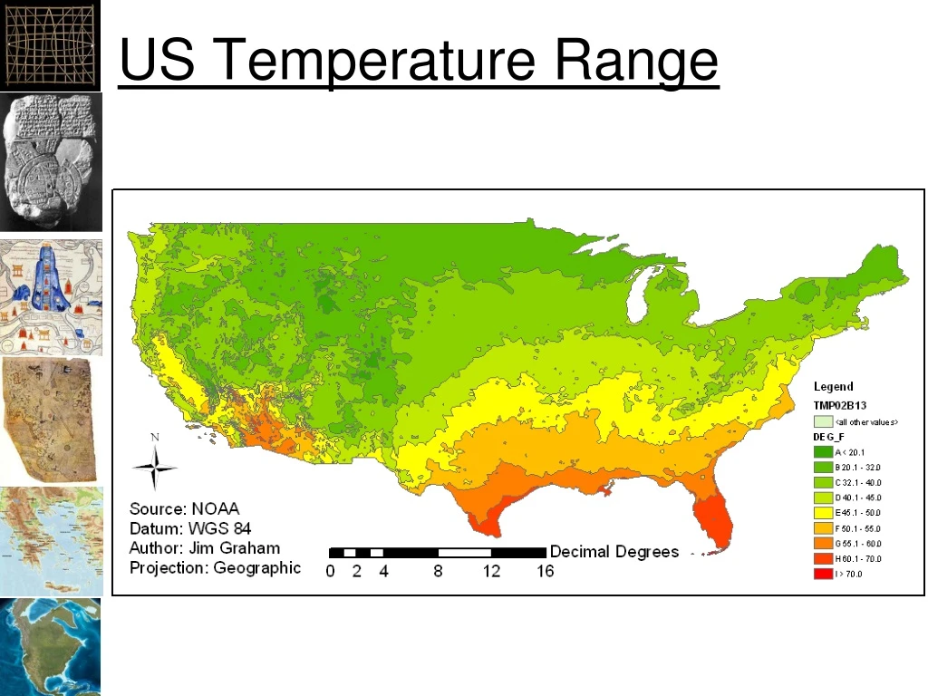

US Temperature Range
E N D
Presentation Transcript
US Weather Stations ~450 km http://www.raws.dri.edu/
Interpolation • Interpolation is a method of constructing new data points within the range of a discrete set of known data points.
Elevation (DEM) Bolstad
First Law of Geography • “Everything is related to everything else, but near things are more related than distant things” • Waldo Tobler
Measuring Autocorrelation • Moran’s I • In ArcMap: Spatial Statistics Tools -> Analyzing Patterns -> Spatial Autocorrelation (Moran’s I) • 0 ~ Random • 1 = Perfect Correlation • -1 = Perfect Dispersion (pattern) ArcGIS Help
Moran’s I • Where: • : number of points indexed by and • : measured value • : mean measured value • : matrix of weights • Example: 1 for neighbors, 0 otherwise • : sum of all weights
Moran’s I Results 0.8 = Spatial Autocorrelation -0.05 = Random -1 = Opposite of autocorrelation
Inverse Distance Weighting • Points closer to the pixel have more “weight” ArcGIS Help
Process • Obtain points with measurements • Evaluate data (autocorrelation) • Interpolate between the points using: • Nearest (Natural) Neighbor • Trend (fitted polynomial) • Inverse Distance Weighting • Kriging • Splines • Density • Convert the raster to vector using contours
Simple Interpolation 50 40 35 Measured Values 20 Spatial Cross-section
Linear Interpolation 50 40 35 Measured Values 20 Spatial Cross-section
Linear Interpolation • Trend surface with order of 1 50 40 35 Measured Values 20 55 47 42 36 36 37 38 40 34 28 21 Spatial Cross-section
ArcToolbox • Simple Interpolation • IDW • Kriging • Natural Neighbor • Spline • Trend • Ok for cartography • Lack the capability of the Geostatistical Wizard
Inverse Distance Weighting • No value is outside the available range of values • Assumes 0 uncertainty in the data • Smooth's the data
Kriging • Semivariograms • Analysis of the nature of autocorrelation • Determine the parameters for Kriging • Kriging • Interpolation to raster • Assumes stochastic data • Can provide error surface • Does not include field data error (spatial or measured)
Semivariance • Variance = (zi - zj)2 • Semivariance = Variance / 2 zj zi - zj zi Distance Point i Point j
Semivariance • For 2 points separated by 10 units with values of 0 and 2: ( 0 – 2 )2 / 2 = 2 2 Semivariance (zi - zj)2 / 2 Distance Between Points 10
Range, Sill, Nugget www.unc.edu
Definitions • Isotropic – Identical in all directions, direction does not matter • Anisotropic – Different in different directions, direction does matter Distribution of galaxies universe advanture.org Trees blown down in St. Helens Eruption www.boston.com
Interpolation Software ArcGIS with Geostatistical Analyst R Surfer (Golden Software) Surface II package (Kansas Geological Survey) GEOEAS (EPA) Spherekit (NCGIA, UCSB) Matlab
More Resources • Geostatistical Analyst -> Tutorial • Wikipedia: • http://en.wikipedia.org/wiki/Kriging • USDA geostatistical workshop • http://www.ars.usda.gov/News/docs.htm?docid=12555 • EPA workshop with presentations on geostatistical applications for stream networks: • http://oregonstate.edu/dept/statistics/epa_program/sac2005js.htm
Literature Lam, N.S.-N., Spatial interpolation methods: A review, Am. Cartogr., 10 (2), 129-149, 1983. Gold, C.M., Surface interpolation, spatial adjacency, and GIS, in Three Dimensional Applications in Geographic Information Systems, edited by J. Raper, pp. 21-35, Taylor and Francis, Ltd., London, 1989. Robeson, S.M., Spherical methods for spatial interpolation: Review and evaluation, Cartog. Geog. Inf. Sys., 24 (1), 3-20, 1997. Mulugeta, G., The elusive nature of expertise in spatial interpolation, Cart. Geog. Inf. Sys., 25 (1), 33-41, 1999. Wang, F., Towards a natural language user interface: An approach of fuzzy query, Int. J. Geog. Inf. Sys., 8 (2), 143-162, 1994. Davies, C., and D. Medyckyj-Scott, GIS usability: Recommendations based on the user's view, Int. J. Geographical Info. Sys., 8 (2), 175-189, 1994. Blaser, A.D., M. Sester, and M.J. Egenhofer, Visualization in an early stage of the problem-solving process in GIS, Comp. Geosci, 26, 57-66, 2000.