Download
1 / 15
160 likes | 402 Vues
data assimilation on a two-layer QG channel model. MPO624 final project Ting-Chi Wu. Data assimilation (1/2). The “Forecast” will be the “First Guess” of the next time step. Objective analysis. Data assimilation (2/2). DA cycle. Error = RMS of (DA run – Truth run)

E N D
data assimilation on a two-layer QG channel model MPO624 final project Ting-Chi Wu
Data assimilation (1/2) • The “Forecast” will be the “First Guess” of the next time step. Objective analysis
Data assimilation (2/2) DA cycle Error = RMS of (DA run – Truth run) DA run starts from t=50day, but Truth run starts from t=100day
2-layer QG channel model • Potential vorticity equation • One variable: streamfunction ~29km ~50km First guess (Background) : day 50 of true run Observation : day 100 of true run
Experiments • DA run: only assimilate upper layer • Direct insertion (no objective analysis) • Int=1day • Int=2day • Int=5day • Optimum Interpolation • Div=2 gridpoints • Div=3 gridpoints • Div=4 gridpoints • Div=5 gridpoints
With random error 5 % of average value
Optimum Interpolation (1/2) Observation True value on gridpoint Analyzed value on gridpoint Use correlation instead of covariance
Optimum Interpolation (2/2) Model gridpoint observation
Optimum Interpolation (2/2) For every gridpoint, pick 8 nearest observations Model gridpoint observation
With Objective Analysis • Model gridpoints: • X=128; Y=65; Points: 8320
After OA (1/3) observation First guess/background Different spatial intervals
Future work • Pick another time-period • Apply other assimilation scheme