Download
1 / 17
170 likes | 261 Vues
This procedure involves using Oliver Kortner's solution to correct drift electron motion in an MDT environment with a B-Field. The process includes computing scalable correction functions based on Garfield, assigning average B-Fields, and creating RT functions for each Chamber. The text outlines first and second-order corrections, coordinates, transformations, and nonlinear corrections. Real data comparisons are conducted using MUTRAK, and the aim is to achieve an overall tube resolution of 94μm. Systematic resolution degradations in various chambers are analyzed, with resolutions evaluated against product comparisons. Suggestions for correction approaches in different chamber types are provided, highlighting areas for improvement and automation.

E N D
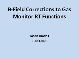
B-Field Corrections to Gas Monitor RT Functions Jason Hindes Dan Levin
Procedure • Use the functional form of Oliver Kortner’s solution to the drift electron’s equation of motion in the MDT environment with a B-Field on • Compute a scalable correction function based on Garfield • Assign an average B-Field to every Chamber from AMDB and a static B-Field map • Compute an RT function for every Chamber
Equation of Motion for Drift Electrons: ; • Solution: • Corrections:
First Order Corrections: • Second Order: • Coordinates: • Effective B-Field that requires correction is • Work out the transformations
Garfield Simulation Correction Function • Garfield • Output TRs in steps of .05T from 0T to1T • Compute all possible combinations of and normalize to reference field. • Use average and cutting procedure to create a scalable correction function from the normalized dTRs.
Residuals: RT(B=0) and Correction Function with RT(B=.5T) Real Data Comparison Using Track Reconstruction Program MUTRAK
Residuals: RT(B=0) and Correction Function with RT(Bx=.3T,By=.3T,Bz=.3T)
Can We Use A Single B-Field Corrected RT Per Chamber? • Assign an average B-Field per Chamber from a line integral along bases with even steps. • Compute the average drift time correction in an MDT at a particular location from the average B-Field and the actual B-Field. • Take the difference between these measurements and multiply by the average drift velocity. This will be the local resolution degradation. • Repeat this process iteratively over the chamber and average the results. This will be the average resolution degradation in a given chamber. • We want this to be less than 50μm: the overall tube resolution will be 94μm.
Systematic Resolution Degradation BI BM BO
Conclusion • The resolution degradation is less than 50μm, in 69% of the chambers. • 87% in the Endcap: Exceptions are EIL4, EEL1, EEL2, EES1,EES2. • 90% in EI, 100% in EM, 100% in EO, and 10% in EE. • 55% in the Barrel: 54% in BI, 63% in BM, and 55% in BO. • Corrections in the Barrel will have to be made at the hit-level. • Endcap corrections could be added to the Automated Temperature Correction Procedure