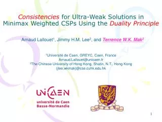
Consistencies for Ultra-Weak Solutions in Minimax Weighted CSPs Using the Duality Principle

1. Consistencies for Ultra-Weak Solutions inMinimax Weighted CSPs Using the Duality Principle Arnaud Lallouet1, Jimmy H.M. Lee2, andTerrence W.K. Mak2 1Université de Caen, GREYC, Caen, France Arnaud.Lallouet@unicaen.fr 2The Chinese University of Hong Kong, Shatin, N.T., Hong Kong {jlee,wkmak}@cse.cuhk.edu.hk

2. Introduction • Motivation • Minimax Weighted CSPs • Ultra-weakly solved, weakly solved, and strongly solved • Consistency Techniques • Lower Bound formulations • Upper Bounds using duality principle • Strengthening lower and upper bounds by adopting WCSP consistencies • Performance Evaluations • Conclusion & Future Work

3. Radio Link Frequency Assignment Problems • Soft Constrained Problems • Model: Weighted CSPs/COPs • CELAR Problem [Cabon et al., 1999]: • Given a set S of radio links located between pairs of sites • Assign frequencies to S: • Prevent/Minimize interferences • Involves two types of constraints CELAR Problem: http://www.inra.fr/mia/T/schiex/Doc/CELAR.shtml

4. Radio Link Frequency Assignment Problems D Communication from A to B B C A Communication from B to A

5. Radio Link Frequency Assignment Problems D Technological constraints |fAB - fBA| = constant B C fAB fBA between two sites A

6. Radio Link Frequency Assignment Problems D fBC B C fCB fAB between links close to each other fBA A Constraints to prevent interferences: e.g. |fAB - fBC| > threshold Sometimes the problem is unfeasible…

7. Radio Link Frequency Assignment Problems D fBC B C fCB fAB between links close to each other fBA A Soft constraints to minimize interferences: e.g. max(0, threshold - |fAB - fBC|)

8. Radio Link Frequency Assignment Problems insecure region Subject to control by adversaries D fBD fDB Minimize interferences? B C Minimize interferences? A

9. Radio Link Frequency Assignment Problems • Nature of the problem: • Optimization: Minimizing interferences • Adversaries: Controlling parts of the links • We can solve: • Many COPs/WCSPs • Each perform optimization on one combination of adversary’s frequency adjustment • Multiple QCSPs • Reducing into a decision problem

10. Radio Link Frequency Assignment Problems • Viewing in game theory: • Two-personzero-sumturn-based game • Allis [1994] proposes three solving levels: • Ultra-weakly solved • Best-worst case for a player • Weakly solved • Strategies for a player to achieve his/her best against all possible moves by his/her opponent • Strongly solved • Strategies for a player to achieve his/her best against all legal moves Our work Stronger

11. Radio Link Frequency Assignment Problems insecure region Assume worst case adversary D fBD Minimize interferences a priori? fDB B C Minimize interferences a posteriori? Minimize interferences a priori? Minimize interferences a posteriori? A Finding frequency assignments for the worst possible case!

12. Minimax Weighted CSPs To avoid multiple sub-problems, we propose: Minimax Weighted CSPs = Min/Max Quantifiers + Soft Constraints + CSPs ≈ Quantified CSPs Weighted CSPs +

13. Minimax Weighted CSPs Minimax Weighted CSP [Lee et al., 2011] Variables: x1, x2, x3 Domains: D1=D3 ={a,b,c}, D2 = {a,b} Soft Constraints: Global Upper Boundk: 11 Valuation structure: ([0..k], ⊕, ≤ ) Quantifier Sequence: Q1 = max, Q2 = min, Q3 = max Soft constraints Unary constraint Binary constraint

14. A-Cost for Sub-problems 4 ⊕ 0 ⊕ 5 ⊕ 1 ⊕ 0 = 10

16. A-Cost for Sub-problems Best-worst case (ultra-weak solution): {x1 = a, x2 = a, x3 = a} A-cost for the problem: 10

17. Algorithms for Ultra-Weak Sol. Previous Work [Lee et al., 2011]: • Alpha-beta prunings • Maintains two bounds • Alpha lb: Best costs for max players • Beta ub: Best costs for min players • Suggest Two sufficient conditions to perform prunings and backtracks Computing the exact A-cost is hard! (NP-hard) Theorem: For the set S of sub-problems P ’, where vi is assigned to xi: ∀P ’ ∈ S, A-cost(P ’) ≥ ub(Condition 1), or ∀P ’ ∈ S, A-cost(P ’) ≤ lb(Condition 2) We can prune or backtrack according to the table:

18. Sufficient Conditions for Prunings How to compute efficiently? Corollary: For the set of sub-problems P’ obtained from P, where vi is assigned to xi: A-cost(P ’) ≥lbaf(P ,xi= vi) ≥ ub(Condition 1), or A-cost(P ’) ≤ ubaf(P ,xi= vi) ≤ lb(Condition 2) We can prune or backtrack according to the table below:

19. Consistencies • Local consistency enforcement • Make implicit costs information explicit • E.g. bounds, prunings/backtracks • Consistencies composes of 3 parts: • Lower bound estimation: lbaf(P ,xi= vi) • NC& AC version • Upper bound estimation:ubaf(P ,xi= vi) • Two dualities: DC & DQ • Strengthening lower & upper estimation by projections/extensions • Adopt WCSP consistencies: NC*, AC*, FDAC* • Naming convention: • DC-NC[proj-NC*], DQ-AC[proj-FDAC*]

20. Lower Bound Estimation • Lower bound estimation: lbaf(P ,xi= vi) • Consider a simplified problem: • Only unary constraints, i.e. no binary Lemma: The A-cost of an MWCSP P with only unary constraints is equal to: Q1C1⊕ Q2C2 ⊕ … ⊕QnCn ⊕ ⊕ = 8 Q1 = max Q2 = min Q3 = max

21. Lower Bound Estimation • Lower bound (NC version): nclb(P ,xi= vi) • Example: • nclb(P ,x1 = b) • nclb(P ,x2 = a) CØ ⊕ (⊕j<i min Cj) ⊕ Ci(vi) ⊕ (⊕i<jQj Cj) Q1 = max Q2 = min Q3 = max For all sub-problems where x2 = a Q1 = max Q2 = min Q3 = max

22. Lower Bound Estimation • Lower bound (AC version): aclb[Cij](P ,xi= vi) • nclb(P ,xi= vi) + a binary constraintCij • Example: • aclb(P ,x1 = b) Q1 = max Q2 = min Q3 = max

23. Upper Bound Estimation • Upper bound ubaf(): Duality of Constraints • Definition of Dual Problem: • Given an MWCSP P = (X,D,C,Q,k). • The dual problem of P is P Τ = (X,D,C Τ,Q Τ,k) where: • Quantifier:Qi = max →Q Τi= min & Qi = min → Q Τi= max • Cost: For a complete assignment l, cost(l) = -1*costΤ(l) Construction Method: -1 Q1 = max Q2 = min -1 Q1 = min Q2 = max

24. Upper Bound Estimation • Upper bound: Duality of Constraints (DC) • Corollary: A lbaf(P Τ,xi= vi) on the dual multiply by -1 is an ubaf(P ,xi= vi) for the original problem lbaf(P Τ,x2= b) ≤ -11 → -1 * lbaf(P Τ,x2= b) ≥ 11

25. Upper Bound Estimation • Following the corollary: • We implement ubaf(P ,xi= vi) by: • NC version: nclb(P Τ,xi= vi) • AC version :aclb[Cij](P Τ,xi= vi) • Advantage for Duality of Constraints (DC) • Reuse the same lbaf() • New lbaf() can be used as ubaf()

26. Upper Bound Estimation • Upper bound: Duality of Quantifiers (DQ) • Creating/Writing new ubaf() via: • Flipping quantifiers of existing lbaf() • Example: • nclb(P ,x2 = a) • ncub(P ,x2 = a) For all sub-problems where x2 = a, guarantee a lower bound Q1 = max Q2 = min Q3 = max For all sub-problems where x2 = a, guarantee an upper bound Q1 = max Q2 = min Q3 = max

27. Upper Bound Estimation • Upper bound: Duality of Quantifiers (DQ) • Creating/Writing new ubaf() via: • Flipping quantifiers of existing lbaf() • Immediate attempt: • Problem: Binary constraints add costs! CØ ⊕ (⊕j<i min Cj) ⊕ Ci(vi) ⊕ (⊕i<jQj Cj) min to max CØ ⊕ (⊕j<imaxCj) ⊕ Ci(vi) ⊕ (⊕i<jQj Cj)

28. Upper Bound Estimation • Upper bound: Duality of Quantifiers (DQ) • Creating/Writing new ubaf() via: • Flipping quantifiers of existing lbaf() • To fix: • Further add maximum costs for constraints which are not covered in the function • For implementation: • We pre-compute and add these maximum costs before search • We maintain the added sum during search CØ ⊕ (⊕j<imaxCj) ⊕ Ci(vi) ⊕ (⊕i<jQj Cj)

29. Consistencies • We have methods to compute: • lbaf(): NC & AC version • Standard approximation analysis • ubaf(): Two dualities • Inspired from QCSP consistencies and algorithms • [Bordeaux and Monfroy, 2002] • [Gent et al., 2005]

30. Consistencies • Can we further strengthen both estimation functions? • Utilize projections & extensions conditions • WCSP consistencies: NC*, AC*, and FDAC* [Cooper et al., 2010] • For Duality of Constraints (DC) consistencies • Conditions are enforced in both the original and dual problem

31. Performance Evaluation • Compare and study different consistency notions • DQ-NC[proj-NC*], DQ-AC[proj-AC*], DQ-AC[proj-FDAC*] • DC-NC[proj-NC*], DC-AC[proj-AC*], DC-AC[proj-FDAC*] • Benchmarks: • Randomly Generated Problems • Graph Coloring Game • Generalized Radio Link Frequency Assignment Problem • Each set of parameters: • 20 instances & taking average result • If there are unsolved instances, we state the #solved besides runtime • Compare our results against: • Alpha-beta pruning • QeCode: A solver for solving QCOP+

32. Performance Evaluation Randomly Generated Problems [Lee et al.,2011] • (n,d,p): (# of vars, domain size, constraint density) • Integer costs of a binary constraint • Generated uniformly in [0…30] for each tuple of assignments • Probability of 50%: a min (max resp.) quantifier • Time limit: 900s Duality of Constraints Extracts costs from two different copies of constraints (original and dual) and resolve the issue • Stronger projection/extension • We may: • Strengtheninglbaf() (ubaf() resp.) • Weakeningubaf() (lbaf() resp.)

33. Conclusion • Define and implement various consistency notions for MWCSPs • Lower bound by costs estimations • Upper bound by duality principle • Strengthening lower & upper bound estimation functions: • Adopting projection/extension conditions in WCSP consistencies • Discussions on our solving techniques on the two other stronger solutions

34. Related Work • Related CSP frameworks tackling adversaries: • Stochastic CSPs [Walsh, 2002] • Adversarial CSPs [Brown et al., 2004] • QCSP+/QCOP+ [Benedetti et al., 2007] [Benedetti et. al, 2008] • Other related frameworks: • Bi-level Programming • Plausibility-Feasibility-Utility framework [Pralet et al., 2009]

35. Future Work • Consistency algorithms: • High-arity Soft Table Constraints, and • Global Soft Constraints • Theoretical comparisons on different consistency notions • Algorithms tackling stronger solutions • Online & Distributed Algorithms • Value ordering heuristics • ICTAI 2012

36. Q & A

37. Performance Evaluation Graph Coloring Game [Lee et al.,2011] • Two player zero-sum games • Writing numbers of nodes • (v,c,d): (# of vertices, # allowed numbers, edge density) • Turns: • Odd/Even numbered turns - Player 1/Player 2 → A series of alternating quantifiers • Time limit: 900s • Similar results

38. Performance Evaluation Generalized Radio Link Frequency Assignment • Designed according to two CELAR sub-instances • Minimize interference beforehand • (i,n,d,r): (CELAR sub-instance index, # of links, # of allowed frequencies, ratio of adversary links) • Time limit: 7200s • Projection/extension in FDAC* • Slightly improves the search only • Quantifier info. not considered

39. Algorithms for Stronger Sol. • Solution Size • Ultra-weak: O(n) • Weak: O((n - m)dm) • Strong: O(dn) • Where: • # of variables: n • # of adversary variables: m • Maximum domain size: d • Ultra-weak solutions are linear

40. Algorithms for Stronger Sol. • Pruning Conditions • A sound pruning condition when solving a weaker solution may not hold in stronger ones • Reason: • Removal of the assumption of optimal/perfect plays • Invalid: • When finding weak solutions • Adversary max player • Invalid: • When finding weak solutions • Adversary min player Theorem: For the set S of sub-problems P ’, where vi is assigned to xi: ∀P ’ ∈ S, A-cost(P ’) ≥ ub(Condition 1), or ∀P ’ ∈ S, A-cost(P ’) ≤ lb(Condition 2) We can prune or backtrack according to the table:

41. Relations with complexity classes • Weighted CSPs: • NP-hard • Quantified CSPs: • PSPACE-complete Theorem: • Finding the truthfulness of QCSPs can be reduced (by Karp reduction) to finding the A-Cost of MWCSPs →MWCSPs: • PSPACE-hard Assumption: P ≠ PSPACE

42. Transforming MWCSP to QCOP • Theorem: • An MWCSP P can be transformed into a QCOP P’. The A-cost of P can be found by solving the optimal strategy of P’. • Proof (Sketch): • Using ‘Soft As Hard’ approach [Petit et. al, 2001] • Transform soft constraints into hard constraints

43. Graph Coloring Game (GCG) Owned by B Owned by A Maximize costs Owned by A Minimize costs Owned by B Player A Player B Owned by B Owned by A Owned by A Owned by B How do they play the game?

44. Graph Coloring Game 5/B 6/A Write number 3 on node 1 Write number 6 on node 2 2/B 1/A Player A Player B 6 3 8/A 7/B 3/A 4/B Game Cost:|3-6|=3

45. Graph Coloring Game 5/B 6/A 2/B 1/A Maximize costs 6 3 Place 0 Gain a cost of 3 Place 3 No cost gain Player A What should I do? 8/A 7/B so on… 3/A 4/B

46. Graph Coloring Game 5/B 6/A When the game terminates… 5 2 1/A 2/B 3 6 What we want to study… 9 1 8/A 7/B 0 5 3/A 4/B Final Game Cost: 55

47. 5/B 6/A Approach 1: 1/A 2/B 8/A 7/B 3/A 4/B so on… 6/A 6/A 0 0 0 6/A 1/A 1/A 1/A 0 0 0 Modeled and solved by COP/ Weighted CSP Modeled and solved by COP/ Weighted CSP Modeled and solved by COP/ Weighted CSP 1 0 1 8/A 8/A 8/A 1 0 0 3/A 3/A 3/A

48. Modeling GCG Approach 2: 5/B 6/A 1/A 2/B 7/B 8/A 3/A 4/B • Guess a threshold: 56 • Generate a Quantified CSP [Bordeaux and Monfroy, 2002] which asks: • Can player A finds numbers against player B’s moves • s.t. Player A gets costs < 56?

49. Modeling GCG • Approach 1: • Number of COPs/ Weighted CSPs constructed is exponential to the possible numbers player B can write • Approach 2: • Generate Quantified CSPs based on the objective function

50. NC Q3 = max Q1 = max Q2 = min AC Merge Q3 = max Q1 = max Q2 = min