Butterfly Network
Butterfly Network. A butterfly network consists of (K+1)2^k nodes divided into K+1 Rows, or Ranks.

Butterfly Network
E N D
Presentation Transcript
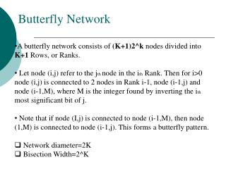
Butterfly Network • A butterfly network consists of (K+1)2^k nodes divided into K+1 Rows, or Ranks. • Let node (i,j) refer to the jth node in the ith Rank. Then for i>0 node (i,j) is connected to 2 nodes in Rank i-1, node (i-1,j) and node (i-1,M), where M is the integer found by inverting the ith most significant bit of j. • Note that if node (I,j) is connected to node (i-1,M), then node (1,M) is connected to node (i-1,j). This forms a butterfly pattern. • Network diameter=2K • Bisection Width=2^K
Example of a Butterfly Network Here is a Butterfly Network for K=3 (0,2) (0,6) Rank 0 i=1, j=2=(010)2, j=(110)2=6 i=2, j=2=(010)2, j=(000)2=0 i=3, j=2=(010)2, j=(011)2=3 Rank 1 (1,0) (1,2) (1,6) Rank 2 (2,3) (2,2) (2,0) Rank 3 (3,3) (3,2)
A butterfly network consists of (K+1)2^k nodes divided into K+1 Rows, or Ranks. • Let node (i,j) refer to the jth node in the ith Rank. Then for i>0 node (i,j) is connected to 2 nodes in Rank i-1, node (i-1,j) and node (i-1,M), where M is the integer found by inverting the ith most significant bit of j. • Note that if node (I,j) is connected to node (i-1,M), then node (1,M) is connected to node (i-1,j). This forms a butterfly pattern. (0110) (0000) (0001) (0010) (0011) (0100) (0101) (0111) (0,6) For K=3 (3+1)2*2*2=32 Total nodes, 32/K+1=32/4=8 Each Rank has 8 nodes (0,2) Rank 0 (i,j) allowing the coordination of Ranks and nodes, i=Rank and j=node in a specific position. Rank 1 (1,2) (1,0) (1,6) (0,2) = (i-1,j) (0,6) = (i-1,M) (2,2) Rank 2 (2,3) (2,0) (1,2) = (i,j) (1,6) =(i,M) Rank 3 (3,3) (3,2)
Cube Connected Cycles • CCC is an unidirected graph, formed by replacing each vertex of a hypercube graph by a cycle • CCC of order n (denoted CCCn) can be defined as a graph formed from a set of n2n nodes, indexed by pairs of numbers (x, y) where 0 ≤ x < 2n and 0 ≤ y < n • Each such node is connected to three neighbors: (x, (y + 1) mod n), (x, (y − 1) mod n), and (x ⊕ 2y, y), where "⊕" denotes the bitwise exclusive or operation on binary numbers
Cont. • An n-cube network has n2n nodes where two nodes are connected if the binary representation of their addresses differs by one and only one bit • Each node can be identified by a pair ( x, y) of integers, where x is the cycle number (the node number in the original hypercube) and y is the node number within the cycle • This same numbering scheme is applicable to the representation below
Transformation of a Hypercube to CCC 0,2 0,0 1,0 0,1 0,1 2,1
Advantages of CCC • The advantage of cube-connected cycles is that the node's degree is always 3, independent of the value of n
Disadvantages • CCC tends to suffer from considerable performance degradation when fault arises
'Trees topologies' are hierarchical structures that have some resemblance to natural trees. Its starts with a node at the top called the root. This node is connected to other nodes by 'edges' or 'branches'. The nodes may spawn further nodes forming a multilayered structure. Introduction to Tree Topology 9
Nodes at one level can only connect to nodes in adjacent levels A node may have only one parent even though it may give rise to several children. Nodes that do not have any children are called 'terminal nodes‘ Figure 1 and 2: below illustrates both the binary and ternary trees. Tree Topology 10
By examining the figures it can be seen that there is only one path between any two nodes. A message from one terminal node to another terminal node has to be routed back up the tree to the first node that is common to both the sender and the receiver. Once the message arrives at the common parent it can then travel back down the tree to the receiving node. Tree Topology 13
An important step in finding the message path involves finding the first node that is common to both sender and receiver This can be done by generating two lists of successive parents all the way up to the root. One list for the sender and one for the receiver The parent of the current node can be found by dividing the address by two and taking the modulus Tree Topology 14
Path finding can be illustrated with reference to figure 3. Let node four be the sender and node ten the receiver. The list of successive parents will be as follows: 15
Message Passed from Node 4 to Node 10 in a Binary Tree Path from Node to Root Sender Receiver Binary Decimal Binary Decimal 0100 4 1010 10 0010 2 0101 5 0001 1 (root) 0010 2 0001 1 (root) 17
It can be seen that the first node to appear in both lists is 2. The path is generated by traversing down the sender list as far as the common node (in this case 2), and then up the receiver list from the common node to the top. A disadvantage of this topology is that there is no alternative route if a necessary link fails. Introduction to X-Tree Topology 18
One way to alleviate this communication problem is to add links between branches at the same level. The resulting structure is called an ‘X-tree‘ . X-tree is an extended tree topology as shown in figure 4 below: Introduction to X-Tree Topology 19
Like the ring, it uses direct connections between processors; each having three connections. There is only one unique path between any pair of processors. The X-tree therefore avoids overlap whenever it is possible without allowing the tree to degenerate. Therefore the Extended-tree (X-tree) topology provides availability of communication between nodes if one link fails. Introduction to X-Tree Topology 21
SHUFFLE EXCHANGE • Consider a set of N processors, numbered P0, P1, … PN-1 • Perfect shuffle connects processors Pi and Pj by a one-way communications link, • If j = 2*i for 0 <= i <= N/2 – 1 or j = 2*i + 1 – N otherwise. • See below an example for N= 8 where arrows represent shuffle links and solid lines represent exchange links.
SHUFFLE EXCHANGE • In other words, perfect shuffle connects processor I with (2*I modulo (N-1)), with the exception of the processor N – 1 which is connected to itself. • Having trouble with this logic • Consider the following:
SHUFFLE EXCHANGE • Let’s represent numbers i and j in binary. • If j can be obtained from i by a circular shift to the left, then Pi and Pj are connected by one-way communications link, viz.:
THE END 27