Download
1 / 62
620 likes | 859 Vues
Building a Structural Dynamic Model of a Boeing 787. Alex Brose, Tanveer Chandok , and Alex Dowgwillo. Introduction Design Process Concepts and rationale Derivation of Model and Transfer Functions System response and implementation . Overview.

E N D
Building a Structural Dynamic Model of a Boeing 787 Alex Brose, TanveerChandok, and Alex Dowgwillo
Introduction • Design Process • Concepts and rationale • Derivation of Model and Transfer Functions • System response and implementation Overview
In today’s changing world, composites are proving to be highly favorable in the building of aerospace components • This is changing the way the structure of the part affects and interacts with the aerodynamic model • In this analysis the group was tasked with analyzing the wing section of a Boeing 787 aircraft Introduction
Finite Element Analysis (FEA) methods are most favorable • Primary objective is to design a model that can describe a physical system of panels on a wing from given force inputs and output deflection • Process throughout this model’s design included the following steps: • Research • Discuss • Make simplifying assumptions • Check validity Design Process
After a lot of research on how to approach designing this model, decided that a state space representation would best describe and model the type of system given’s behavior • Why State Space? • System has many degrees of freedom (6 panels) • If we define the system of panels’ FBDs in a “state space manner”, we find that it meets the requirements! Concepts/Rationale
Requirements of State Space • Must be able to be defined as a first order differential equation • First order derivative is a linear combination of “state variables” ie () • State variables are linearly independent of one another State Space Fundamentals
Governing equations of state space: • In equations above, vector is the state vector, is the derivative vector, and is the system matrix (contains coefficients of state variables) • After finding , we can find output vector State Space Fundamentals
As in any system design, we begin the process by doing FBDs and a dynamical analysis… • Note in schematic, is shown as an absolute value, which is what our desired output for the user will take in. In the equations of motion however, it is relative to the previous panel • **Note that twist and vertical deflection will be modeled completely separately. We begin here with vertical deflection • As seen in diagram, all interactions between panels are modeled as torsional spring and damper Moments with some coefficients of and Derivation of Model
Now we write an equation of motion for one of the panels to see what we can work with: • Where is the moment of inertia of panel two, L is aerodynamic lift concentrated at center of panel 2, W is weight of panel 2 (at center), and S is the shear located at the right hand side of each panel • Equations of motion for other panels are found in the same way • Now the next step is to define state variables to be represented in state space Derivation of Model
In Equation of motion we see is a linear combination of all the and terms and those terms are also independent of one another! We can set those as state variables • So lets let so that • With these definitions, we recall: • Where is a vector of all state variables in the system Derivation of Model
For our model: and Derivation of Model
We know that all of the values in our system matrix are the coefficients of the state variables and are values that should be given by the 787 specifications. We define • where is the panel number • here the factor .01 is attained through a process to approximate the damping ratio to be System Matrix
The process suggested by Brad Sexton of Boeing, was to approximate , and work backwards to attain a factor of that yields a reasonable value • We recall that and are related usuallyby some factor • We set and multiply the stiffness matrix (of ) by best guess factors until we achieve a value closest to , and se that factor as our damping coefficient . • Assuming , we can algebraically arrive at System Matrix
Now to approximate and to get the value and our system matrix will be complete! • Using an online source(http://ascelibrary.org/cco/resource/1/jccof2/v8/i2/p141_s1?isAuthorized=no), for carbon composite material through whole wing • For , a structural chord and skin thickness method were used to simplify the geometry, so that airfoil equations are not needed, and instead a rectangle modeling the same bending strength is used System Matrix
Breakpoint • We begin by defining specifications provided by an online source • Where root is cross section at fuselage, break is the breakpoint cross section (shown below) System Matrix
Our goal now is to obtain average values of and that we can use to define an each panel’s cross section • Now, we use algebra to determine linear piece-wise equations for and as a function of span. They are piecewise, because and vary differently after the breakpoint along the span * * System Matrix
Using these equations, and a set vector of span values (5x15ft panels ad 1x14ft panel) we can find an average and value for each panel • Each number above, from left to right, represents average values from panel 1 to 6 • Now that we have averages to work with, we will continue using this “box method” to find our moment of inertia System Matrix
From the same website, the structural chord is defined to be between 15% and 75% of the chord, so all we do here to obtain the “length” of the rectangle is simply scale down the vector by 0.6. So we define a new chord, • – for each panel • For the thickness of this idealized box cross section, the average thickness at the root is estimated but should be scaled down accordingly along the span as the thickness decreases • To do this, a volume ratio, of the panel volume to the entire wing volume was used to scale down the skin thickness estimation System Matrix
For volume ratios, we do not need airfoil equation data, because it is the same for each panel and the whole wing • Our average and vectors are used to determine , the volume of each panel (without airfoil data) -Now we need a representation of the of the whole wing • We now need to define new vectors for and . We can do this in the same manner as before, by using our and equations as function of span * * System Matrix
For better precision we average 7 values of and along the span (at 0, 15, 30, 45, 60, 75,89) and obtain: and • So now the wing volume is: • Now we solve for a vector of volume ratios that we can use to scale down the skin thickness for our box cross section - for the 6 panels • Note this combination of volume ratios does add up to slightly more than 1, so there is some error associated with the and equations used System Matrix
Continuing with the skin thickness assumption estimation, the team estimated the root cross section to be 0.0417 • This skin thickness approximation allows us to use superposition later since we will know the moment of inertia of both shapes(original and accounting for the skin thickness shown here) and will allow us to utilize the assumption that bending strength is generally at the skin • Scaling down the span: -for each panel • Now we have enough to define a value of the moment of inertia of each panel! System Matrix
The moment of inertia for a rectangle is defined to be: - for initial area - for the thickness rectangle • Because we have assumed bending strength comes from the skin, we will use superposition principle to obtain the value for each panel -for each panel • Now we can define the stiffness of each panel! System Matrix
From earlier: • So we have: (lbf*ft) • Now that we know the stiffness, our system matrix for the vertical deflection is defined! (because all values are just 0.1*) • Now the system Matrix is defined by these values! We just use and what we know from the equations of motion to create A and put it into the MATLAB code System Matrix
We are nearly complete creating the vertical deflection state space model for this Boeing 787 wing • To model the input, we must consider all forces on each panel again and define what state variables and their corresponding coefficients are • And the corresponding equation of motion for the case of panel one that we can generalize: Input Matrix
As we can see from the equation of motion, the Lift force (to be given by an aerodynamic model by another team) and the weight, and shear forces are our only inputs • We will define to be an input vector, similar to that we can represent with our state space equation • and then we find Input Matrix
To complete the state space model we need to define our output vector and output matrix. The feedforward matrix is assumed to be zero, because no inputs have a direct effect on the desired output transformation • We now know the x vector, which is the deflection of each panel in radians. But our desired output specifies a vertical deflection in feet. • Assuming small angles, we can just multiply by . Output Matrix
For system response testing and validation procedures, we will have two output components of , one that will output the relative deflection with respect to the previous panel, and one that outputs the absolute deflection with respect to the root at the fuselage of the aircraft • So Output Matrix
Using MATLAB’s “ss2tf” command we can determine the transfer functions of this system • For panel 1, the following transfer function is displayed as an example of what is obtained from these state space representations of this system of panels for the vertical deflection in MATLAB • All of the other transfer functions for each panel are obtained the same way • Take note of the order of this transfer function. It is due to the fact this system of 6 panels interact and affect all other panels. This confirms that state space representation is the best way to approach the problem as opposed to the classical approach Transfer Functions for Vertical Deflection
We have just derived our state space model for the vertical deflection, but we must now include the wing twist • Just as before, we begin with basics on a different FBD. This time our input is a given moment from the aerodynamic model • Input is the input moment. All other interactions between panels are modeled as both a spring and damper torque Derivation of Model (Torsional)
We obtain an equation of motion from the FBD for panel 1 as follows: • Now to get this into the state space domain, we define state variables and such that • Now we define the state vectors and that we can form into our general state space equation: • - where is the torsional input vector • and Derivation of Model (Torsional)
Next we must model the system matrix that corresponds to our chosen state variables and equation of motion for the twist of each panel. • Note: the angle of each panel is taken with respect to the previous panel. is taken with respect to the root, which is assumed horizontal • The system matrix, defined , can be again defined by the physical property coefficients that we see in the equation of motion that correlate to each of our state variables System Matrix (Torsional)
The torsional system matrix has the same type of values as the vertical system matrix. Here we have: • -the torsional stiffness - the damping coefficient • Where is the torsional modulus of elasticity for the particular material the Boeing 787 wing is made of • is the moment of inertia of each panel for the twisting, torsional motion, this will again depend on thickness and chord length, similar to how we defined in the vertical system matrix System Matrix (Torsional)
, the damping coefficient is again found approximated in the same manner as before. The damping ratio is assumed to be close to from Mr. Sexton • We recall that and are related usually by some factor • We set and multiply the stiffness matrix (of ) by best guess factors until we achieve a value closest to , and se that factor as our damping coefficient . • Assuming , we can algebraically arrive at System Matrix (Torsional)
To define , we make a series of very similar assumptions about the airfoil size and shape as before • Using online sources(http://www.engineeringtoolbox.com/young-modulus-d_417.html) • For , we will assume the same “box” shape approximation of the airfoil shape System Matrix (Torsional)
Recall: • And: • -for each panel • We arrive at these approximations using the assumption that bending strength comes from the skin, which we assume to be a box around the structural chord, System Matrix (Torsional)
So now using this values and approximations of thickness for airfoil cross section characteristics: • -general form • We will use the superposition principle again to account for our skin thickness simplification • – for each panel System Matrix (Torsional)
Now we have all the terms to define our and also values! • -the torsional stiffness - the damping coefficient (lbf*ft) (lbf*ft) System Matrix (Torsional)
So now for the state space relation: • Again using linear algebra we can define the system matrix using the physical properties of the wing panels System Matrix (Torsional)
We must now define the input matrix and our state space model for wing twist will be complete! • From FBD **insert**, we see that we have a pitching moment input acting about the quarter chord point, and that is our only input of interest in this direction of motion • So we will define: • -where is the aero moment input at the respective panel Input Matrix (Torsional)
So for we have: Input Matrix (Torsional)
The next step is finding our output matrix, and then output vector. Using: • And also keeping in mind that the client requested specifically an output with TOTAL twist for every panel, we can define the Matrix to give us the that will meet our requirements Output Matrix (Torsional)
For purposes of validation and system response testing, we are interested in both the twist of each panel with respect to the previous panel, and outputs of the twist of each panel with respect to initial root at fuselage • So • Note that the top half of the matrix assigns the output vector a relative twist value (simply using a radian to degree transformation), while the bottom half uses the same transformation to assign absolute twist of each panel Output Matrix (Torsional)
After Defining all the matrices of the system (A,B,C, and assuming zero for D), we are ready to convert this state space representation into a useful MATLAB transfer function again via the “ss2tf” command • Notice this transfer function is the same exact order as the vertical deflection transfer function. This is because both seek an output vector with same dimension (hence same dimension Matrix) and also same dimension system matrix and state vectors Transfer Functions for Vertical Deflection
The model obtained is tested by using different types of input. Mainly: • Impulse input • Step Input • Sinusoidal input • Turbulent Flow • Steady State Flow System Response and Implementation
The system response produces the following types of outputs: • Deflection vs. Time graphs • BODE plots System Response Outputs
Deflection vs. Time for an Impulse Input. Input is applied on Panel 3 and the resulting deflections on all other panels are displayed. Note how every panel reacts differently due to the changes in the k and b values of each panel Impulse Inputs
2 Impulse Inputs applied on Panel 3 and Panel 5 and 2 Impulse Inputs on the Aileron at 5 deg and 10 deg. The resultant deflections of all other panels is shown. Note: The compounding deflections across the entire wing is noticed. Impulse Inputs
Total tip deflection under Impulse Input on Panel 3: Notice how the system returns back to zero due to the damping effect. Impulse Input
Sinusoidal input on Panel 4. Resultant deflections of every other panel is displayed. Sinusoidal Input
Total deflection of the tip when a Sinusoidal Input at Panel 4 is applied. Sinusoidal Input