Download
1 / 61
610 likes | 786 Vues
A Stackelberg Strategy for Routing Flow over Time. Umang Bhaskar , Lisa Fleischer Dartmouth College Elliot Anshelevich Rensselaer Polytechnic Institute. Traffic Routing. Road network. Data network. Traffic Routing. Safe zone. Evacuation planning. Traffic Routing. Routing Delays.

E N D
A Stackelberg Strategy for Routing Flow over Time UmangBhaskar, Lisa Fleischer Dartmouth College Elliot Anshelevich Rensselaer Polytechnic Institute
Traffic Routing • Road network • Data network
Traffic Routing Safe zone • Evacuation planning
Routing Delays delay • Delay on edges increases with usage delay
Optimal Routing delay • Delay on edges increases with usage delay • Optimalrouting minimizes f(delay)
Uncoordinated Routing delay • But players choose route independently delay
Routing Games delay • Each player picks route to minimize delay • Delays depend on other players delay
Equilibria • Equilibrium: - every player minimizes delay w.r.t. others - no player can unilaterally reduce delay • Studied in many contexts
Price of Anarchy quality of equilibria • How does equilibrium compare to optimal routing? • Price of Anarchy • (PoA) f(delay) of worst equilibria = f(delay) of optimal routing measures system efficiency
Static Flows • Most routing games assume static flows • Static: time-invariant xe xe s t xe
Flows over Time • Edges have fixed capacities and delays • Flow on an edge may vary with time ce, de s t
Flows over Time B A c = 100 bps d = 2 seconds M = 1000 bits Arrival graph: Total time: 12 seconds 100 Quickest flow: flow that gets to destination as soon as possible Bits per second 1 2 3 4 5 6 7 8 9 10 11 12 Time
Temporal Routing Games B A c = 100 bps d = 2 seconds M = 1000 bits • Routing Games + Flows over Time = Temporal Routing Games • Player minimizes time it reaches destination
Temporal Routing Games • Assumptions: • Players are infinitesimal t s M • Model: • Players are ordered at s • Each player picks a path from s to t • Minimizes the time it arrives at t Arrival Graph: M Flow rate at t Time
Temporal Routing Games Flow rate at t c = 1, d = 1 2 1 s t c = 2, d = 0 v c = 1, d = 0 M Time
Temporal Routing Games Flow rate at t c = 1, d = 1 Queue 2 1 s t c = 2, d = 0 v c = 1, d = 0 M Time
Temporal Routing Games Flow rate at t c = 1, d = 1 Queue 2 1 s t c = 2, d = 0 v c = 1, d = 0 M Time • Queues grow when inflow exceeds capacity on an edge • Queues are first in, first out (FIFO) • Queuing models used in modeling traffic [Vickrey ‘69, Yagar ‘71]
Temporal Routing Games Flow rate at t c = 1, d = 1 2 1 s t c = 2, d = 0 v c = 1, d = 0 M Time
Temporal Routing Games Flow rate at t c = 1, d = 1 2 1 s t c = 2, d = 0 v c = 1, d = 0 M Time
Temporal Routing Games Flow rate at t c = 1, d = 1 2 1 s t c = 2, d = 0 v c = 1, d = 0 M Time
Temporal Routing Games Flow rate at t c = 1, d = 1 M 2 1 s t c = 2, d = 0 v c = 1, d = 0 M Time
Temporal Routing Games Flow rate at t c = 1, d = 1 M 2 1 s t c = 2, d = 0 v c = 1, d = 0 M Time Quickest Flow: Flow rate at t M c = 1, d = 1 2 fp = 1 1 s t v M fp = 1 c = 2, d = 0 c = 1, d = 0 Time
Temporal Routing Games Flow rate at t c = 1, d = 1 M 2 1 s t M c = 2, d = 0 v c = 1, d = 0 Time our case • For single-source, single sink, equilibrium exists • [Koch, Skutella, ’09; Cominetti, Correa, Larre ‘11] • How does equilibrium in these games compare with optimal? • What is the PoA?
Objectives M’ =? Evacuation Price of Anarchy: Flow rate at t |Flow| reaching t by time T Time T Flow rate at t Time Price of Anarchy: M Time for M to reach t ? Time ∫ = ? Total Delay Price of Anarchy: Flow rate at t Sum of times for M to reach t Time ? Maximum delay of a player Flow rate at t Time
Results M’ = ? Evacuation Price of Anarchy: Ω(log n) [KS ‘09] Flow rate at t |Flow| reaching t by time T Time T Flow rate at t Time Price of Anarchy: ≥e/(e-1) [KS ‘09] M Time for M to reach t ? Time ∫ = ? Total Delay Price of Anarchy: Flow rate at t Sum of times for M to reach t Time ? Ω(n) [MLS ‘10] Maximum delay of a player Flow rate at t Time
Results Our Results M’ = ? Evacuation Price of Anarchy: Ω(log n) [KS ‘09] Flow rate at t |Flow| reaching t by time T Time T Flow rate at t Time Price of Anarchy: ≥e/(e-1) [KS ‘09] M Time for M to reach t = e/(e-1) † ? Time ∫ =? Total Delay Price of Anarchy: Flow rate at t = 2 e/(e-1) † Sum of times for M to reach t Time ? Ω(n) [MLS ‘10] Maximum delay of a player Flow rate at t †can be enforced by reducing capacities Time
Temporal Routing Games • Main Result: Can enforce bound of e / (e-1) on Time PoA by reducing edge capacities M ? • Procedure: - compute quickest flow (can compute in poly time [FF ’62]) - reduce edge capacities to that used by quickest flow c = 1, d = 1 fp = 1 v w s t c = 2, d = 0 c = 1.5 , d = 0 c = 1, d = 0 fp = 1
Temporal Routing Games • Main Result: Can enforce bound of e / (e-1) on Time PoA by reducing edge capacities M ? • Procedure: - compute quickest flow (can compute in poly time [FF ’62]) - reduce edge capacities to that used by quickest flow c = 1, d = 1 fp = 1 v w s t c = 2, d = 0 c = 1 , d = 0 c = 1, d = 0 fp = 1
Temporal Routing Games • Main Result: Can enforce bound of e / (e-1) on Time PoA by reducing edge capacities M ? • Procedure: - compute quickest flow (can compute in poly time [FF ’62]) - reduce edge capacities to that used by quickest flow • Main Theorem: If quickest flow saturates graph, then Time PoA ≤ e / (e-1)
Temporal Routing Games If quickest flow saturates graph, then TimePoA ≤ e / (e-1) Theorem 1: M ? Can enforce bound of e / (e-1) on TimePoA by reducing edge capacities ∫ = ? If quickest flow saturates graph, then Total DelayPoA ≤ 2e / (e-1) Theorem 2: Can enforce bound of 2e / (e-1) on Total DelayPoA by reducing edge capacities
Talk Outline For this talk: • Structure of Quickest flow • Structure of equilibria • Sketch weaker version of Theorem 1.
Quickest Flows Flow rate at t OPT: c = 1, d = 1 2 1 s t Time v M c = 2, d = 0 c = 1, d = 0 • Quickest flow is static flow repeated over time [FF ‘62]
Quickest Flows Flow rate at t OPT: c = 1, d = 1 2 1 s t Time v fp = 1 M c = 2, d = 0 c = 1, d = 0 • Quickest flow is static flow repeated over time [FF ‘62]
Quickest Flows Flow rate at t OPT: c = 1, d = 1 2 fp = 1 1 s t Time v fp = 1 M c = 2, d = 0 c = 1, d = 0 • Quickest flow is static flow repeated over time [FF ‘62]
Phases in Equilibria Flow rate at t c = 1, d = 1 Queue 2 1 s t M c = 2, d = 0 v c = 1, d = 0 Time
Phases in Equilibria Flow rate at t c = 1, d = 1 2 1 s t M c = 2, d = 0 v c = 1, d = 0 Time
Phases in Equilibria Flow rate at t c = 1, d = 1 2 1 s t M c = 2, d = 0 v c = 1, d = 0 Time
Phases in Equilibria • Equilibrium proceeds in “phases” [KS ‘09] • Phase characterized by • edges being used • edges with queue • Within phase, flow rate at t is fixed
1-Phase Equilibrium For this talk: For one-phase equilibrium, Time PoA ≤ 2 • Quickest flow • Phases in equilibria • Sketch of proof
A Bound on EQ Arrival Graphs: c = 1, d = 1 Flow rate at t Equilibrium ce = 1 s t c = 2, d = 0 v c = 1, d = 0 Time M EQ M
A Bound on EQ Arrival Graphs: c = 1, d = 1 Flow rate at t Equilibrium ce = 1 s t c = 2, d = 0 v c = 1, d = 0 Time M EQ M c = 1, d = 1 fp = 1 Quickest Flow Flow rate at t co = 2 s t v fp = 1 c = 2, d = 0 c = 1, d = 0 OPT Time
A Bound on EQ Arrival Graphs: c = 1, d = 1 Flow rate at t Equilibrium ce = 1 s t c = 2, d = 0 v c = 1, d = 0 Time M EQ M c = 1, d = 1 fp = 1 Quickest Flow Flow rate at t co = 2 s t v fp = 1 c = 2, d = 0 c = 1, d = 0 OPT co Time Claim 1: ce EQ ≤ co OPT EQ ≤ OPT ce
A Second Bound on EQ Arrival Graphs: c = 1, d = 1 Flow rate at t Equilibrium ce = 1 s t c = 2, d = 0 v c = 1, d = 0 Time EQ
A Second Bound on EQ Arrival Graphs: c = 1, d = 1 Flow rate at t Equilibrium ce = 1 s t c = 2, d = 0 v c = 1, d = 0 Time EQ
A Second Bound on EQ Arrival Graphs: c = 1, d = 1 Flow rate at t Equilibrium ce = 1 s t c = 2, d = 0 v c = 1, d = 0 τ(θ) increasing Time EQ τ(θ) : minimum time taken to reach t at time θ
A Second Bound on EQ Arrival Graphs: c = 1, d = 1 Flow rate at t Equilibrium ce = 1 s t c = 2, d = 0 v c = 1, d = 0 τ(θ) increasing Time EQ τ(θ) : minimum time taken to reach t at time θ co - ce Claim 2: τ(EQ) ≥ EQ co
A Second Bound on EQ Arrival Graphs: c = 1, d = 1 Flow rate at t Equilibrium ce = 1 s t c = 2, d = 0 v c = 1, d = 0 τ(θ) increasing Time EQ τ(θ) : minimum time taken to reach t at time θ co - ce Claim 2: τ(EQ) ≥ EQ co • But graph has path p of length ≤ OPT not being used (ce < co) • When τ(θ) ≥ OPT, this path p should be used (phase ends)
A Second Bound on EQ Arrival Graphs: c = 1, d = 1 Flow rate at t Equilibrium ce = 1 s t c = 2, d = 0 v c = 1, d = 0 τ(θ) increasing Time EQ τ(θ) : minimum time taken to reach t at time θ co - ce co - ce Claim 2: θ ≥ EQ Claim 3: τ(EQ) ≤ OPT Claim 2: τ(EQ) ≥ EQ co co • But graph has path p of length ≤ OPT not being used (ce < co) • When τ(θ) ≥ OPT, this path p should be used (phase ends)
A Second Bound on EQ Arrival Graphs: c = 1, d = 1 Flow rate at t Equilibrium ce = 1 s t c = 2, d = 0 v c = 1, d = 0 τ(θ) increasing Time EQ τ(θ) : minimum time taken to reach t at time θ co - ce + Claim 3: τ(EQ) ≤ OPT Claim 2: τ(EQ) ≥ EQ co co Claim 4: EQ ≤ OPT co - ce