Maximizing Computer Performance: Benchmarking Methods & Weighted Averages
Understand computer performance evaluation through benchmarks & weighted averages for accurate analysis. Learn CPI calculation and ways to improve latency and bandwidth for optimized operations.

Maximizing Computer Performance: Benchmarking Methods & Weighted Averages
E N D
Presentation Transcript
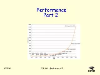
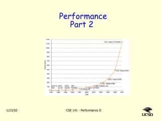
PerformancePart 2 CSE 141 - Performance II
How do you judge computer performance? • Clock speed? • No • Peak MIPS rate? • No • Relative MIPS, normalized MFLOPS? • Sometimes (if program tested is like yours) • How fast does it execute MY program • The best method! Unless ISA is same CSE 141 - Performance II
Benchmarks • It’s hard to convince manufacturers to run your program (unless you’re a BIG customer) • A benchmark is a set of programs that are representative of a class of problems. • Microbenchmarks – measure one feature of system • e.g. memory accesses or communication speed • Kernel – most compute-intensive part of applications • e.g. Linpack and NAS kernel b’marks (for supercomputers) • Full application: • SPEC (int and float) (for Unix workstations) • Other suites for databases, web servers, graphics,... CSE 141 - Performance II
The SPEC benchmarks SPEC = System Performance Evaluation Cooperative (see www.specbench.org) • A set of “real” applications along with strict guidelines for how to run them. • Relatively unbiased means to compare machines. • Very often used to evaluate architectural ideas • New versions in 89, 92, 95, 2000, 2004, ... • SPEC 95 didn’t really use enough memory • Results are speedup compared to reference machine • SPEC 95: Sun SPARCstation 10/40 performance = “1” • SPEC 2000, Sun Ultra 5 performance = “100” • Geometric mean used to average results CSE 141 - Performance II
SPEC89 and the compiler Darker bars show performance with compiler improvements (same machine as light bars) CSE 141 - Performance II
The SPEC CPU2000 suite • SPECint2000 – 12 C/Unix or NT programs • gzip and bzip2 - compression • gcc – compiler; 205K lines of messy code! • crafty – chess program • parser – word processing • vortex – object-oriented database • perlbmk – PERL interpreter • eon – computer visualization • vpr, twolf – CAD tools for VLSI • mcf, gap – “combinatorial” programs • SPECfp2000 – 10 Fortran, 3 C programs • scientific application programs (physics, chemistry, image processing, number theory, ...) CSE 141 - Performance II
SPEC on Pentium III and Pentium 4 What do you notice? CSE 141 - Performance II
Weighted Averages Average of x1, x2, ..., xn is (x1 + x2 + ... + xn) /n This is a special case of weighted average were all the “weights” are equal. Suppose w1, w2, ..., wn are the relative frequency of the xi’s. Assume w1 + w2 + ... + wn = 1. The wi‘s are called weights. The weighted average of the xi‘s is: w1 x1 + w2 x2 + ... + wn xn CSE 141 - Performance II
Weighted Average Example Suppose for some store, 50% of the computers sold cost $700 30% cost $1000 20% cost $1500 The fractions .5, .3 and .2 are weights. The average cost of computers sold is .5 x $700 + .3 x $1000 + .2 x $1500 = $950 The average cost x number sold = total $$ CSE 141 - Performance II
Weighted averaging pitfall The units of the numbers being averaged must correspond to what the weights represent. Specifically, if the units are “A’s per B” (e.g. $/computer) then the weights should be fractions of B’s (computers, in the example). CSE 141 - Performance II
CPI as a weighted average Earlier, I said CPI was derived from time, #instruction, and cycle time. But if you know fraction of instructions that required k cycles (for all relevant k’s) you can calculate CPI using weighted average. CSE 141 - Performance II
CPI as a weighted average Suppose 1 GHz computer ran short program: Load (4 cycles), Shift (1), Add (1), Store (4). We have ½ instructions are CPI=4, ½ are CPI=1. So weighted average CPI = ½ 4 + ½ 1 = 2.5 Time = 4 instructions x 2.5 CPI x 1 ns = 10 ns But 8/10 of cycles have CPI = 4, 2/10 have CPI = 1. Average CPI = 8/10 x 4 + 2/10 x 1 = 3.4 Time = 4 ins x 3.4 CPI x 1 ns = 13.6 ns Which is right? Why ??? L L L L SAS S S S CSE 141 - Performance II
Improving Latency • Latency is (ultimately) limited by physics. • e.g. speed of light • Some improvements are incremental • Smaller transistors shorten distances. • To reduce disk access time, make disks rotate faster. • Improvements often require new technology • Replace stagecoach by pony express or telegraph. • Replace DRAM by SRAM. • Once upon a time, bipolar or GaAs were much faster than CMOS. • But incremental improvements to CMOS have triumphed. CSE 141 - Performance II
Improving Bandwidth • You can improve bandwidth or throughput by throwing money at the problem. • Use wider buses, more disks, multiple processors, more functional units ... • Two basic strategies: • Parallelism: duplicate resources. • Run multiple tasks on separate hardware • Pipelining: break process up into multiple stages • Reduces the time needed for a single stage • Build separate resources for each stage. • Start a new task down the pipe every (shorter) timestep CSE 141 - Performance II
Pipelining • Modern washing machine: • Washing/rinsing and spinning done in same tub. • Takes 15 (wash/rinse) + 5 (spin) minutes • Time for 1 load: 20 minutes • Time for 10 loads: 200 minutes • Old fashioned washing machine: • Tub for washing & rinsing (15 minutes) • Separate spinner (10 minutes) • Time for 1 load: 25 minutes • Time for 10 loads: 160 minutes (25 minutes for first load, 15 minutes for each thereafter) CSE 141 - Performance II
Parallelism vs pipelining Both improve throughput or bandwidth • Automobiles: More plants vs. assembly line • I/O bandwidth: Wider buses (e.g. parallel port) vs. pushing bits onto bus faster (serial port). • Memory-to-processor: wider buses vs. faster rate • CPU speed: • superscalar processor– having multiple “functional units” so you can execute more than one instructions per cycle. • superpipelining– using more steps than “classical” 5-stage pipeline • recent microprocessors use both techniques. CSE 141 - Performance II
Latency vs Bandwidth of DRAM • I claim, “DRAM is much slower than SRAM” • Perhaps 30 ns vs 1 ns access time • But we also hear, “SDRAM is much faster than ordinary DRAM” • e.g. “RDRAM (from Rambus) is 5 times faster...” • Are S(R)DRAM’s almost as good as SRAM? CSE 141 - Performance II
What are limits? • Physics: speed of light, size of atoms, heat generated (speed requires energy loss), capacity of electromagnetic spectrum (for wireless), ... • Limits with current technology: size of magnetic domains, chip size (due to defects), lithography, pin count. • New technologies on the horizon: quantum computers, molecular computers, superconductors, optical computers, holographic storage, ... • Fallacy – improvements will stop • Pitfall – trying to predict > 5 years in future CSE 141 - Performance II
Amdahl’s Law • Suppose: total time = time on part A + time on part B, you improve part A to go p times faster, • then: improved time = time on part A/p + time on part B. • The impact of an improvement is limited by the fraction of time affected by the improvement. new speed/old = (tA+tB)/(tA/p + tB) < (tA+tB)/tB < 1/fraction of unaffected time Moral: Make the common case fast!! CSE 141 - Performance II
A challenge for the future • Latency of moving data to processor is hard to improve. • Processors are getting faster. • Processors must “tolerate latency” • Request data longer before its needed • Find something else to do while waiting. CSE 141 - Performance II
Key Points • Be careful how you specify performance • Execution time = instructions *CPI *cycle time • Use real applications to measure performance • Throughput and latency are different • Parallelism and pipelining improve throughput CSE 141 - Performance II
Computer(s) of the day • One-of-a-kind computers of the 1940’s. • 1941: Z3 - Konrad Zuse (Germany) • programmable, special purpose, relays; • lost funding from Hitler • 1943: Colossus – Alan Turing et al. • special purpose electronic computer; won WWII • Early 1940’s: ENIAC – Eckert & Mauchley at U. Penn • general purpose; conditional jumps; • programmed via plug cables • 80 feet long, 18,000 vacuum tubes, 1900 10-digit adds/sec • 1949: EDSAC – Cambridge England • first full-scale, operational, stored-program computer CSE 141 - Performance II