Unlocking the Potential: Quantum Computing Applications and Algorithms
610 likes | 734 Vues
Explore the capabilities of quantum computing, from elementary gates to quantum parallelism and interference. Learn about Quantum Circuits, Simon's Problem, and the power of Quantum Algorithms. Discover how quantum computing revolutionizes computational tasks through unique concepts like quantum parallelism and the Hadamard transform.

Unlocking the Potential: Quantum Computing Applications and Algorithms
E N D
Presentation Transcript
Quantum Computing:What’s It Good For? Scott Aaronson Computer Science Department, UC Berkeley January 10, 2002 www.cs.berkeley.edu/~aaronson Stacy Seitz John Bell
Elementary gates • Hadamard gate • Phase shift
Elementary gates • Rotation by angle • Controlled NOT
Universality • Any quantum computation can be performed by a circuit consisting of Hadamard, phase, rotation by /8and controlled NOT gates.
Classical vs. Quantum Circuits We can transform a classical circuit for F to quantum circuit. |x> |x> F |0> |F(x)> Add extra input initialized to 0.
|a> |a(xy)> Example Quantum Classical x y |x> |x> |y> |y> ^ |0> |xy> Toffoli gate.
Quantum parallelism • By linearity, • Many evaluations of f in unit time. |x> |x> |0> |f(x)> |x> |f(x)> |x> |0> x x
Quantum parallelism • Once we measure • we get one particular x and f(x). • Same as if we evaluated f on a randomx. |x> |f(x)> x
Quantum parallelism • Is it useful? • We cannot obtain all values f(x) from because quantum states cannot be measured completely. • We can obtain quantities that depend on many f(x). |x> |f(x)> x
Quantum interference • Hadamard transform: Illustrate this with Bloch Sphere
Quantum interference • Negative interference: |1> and -|1> cancel out one another. • Positive interference: |0> and |0> add up to a higher probability. • Use quantum parallelism to compute many f(x). • Use positive interference to obtain information that depends on many values f(x). • Ideal for number-theoretic problems (factoring).
Hadamard matrix: H|0 = (|0+|1)/2 H|1 = (|0-|1)/2 H(|0+|1)/2 = |0 H(|0-|1)/2 = |1
Quantum Circuits • Unitary operation is local if it applies to only a constant number of bits (qubits) • Given a yes/no problem of size n: • Apply order nk local unitaries for constant k • Measure first bit, return ‘yes’ iff it’s 1 • BQP: class of problems solvable by such a circuit with error probability at most 1/3 • (+ technical requirement: uniformity)
The Power of Quantum Computing • Bernstein-Vazirani 1993: BPP BQP PSPACE BPP: solvable classically with order nk time PSPACE: solvable with order nk memory • Apparent power of quantum computing comes from interference • Probabilities always nonnegative • But amplitudes can be negative (or complex), so paths leading to wrong answers can cancel each other out
Simon’s Problem Given a black box f(x) x Promise: There exists a secret strings such that f(x)=f(y) y=xs for all x,y (: bitwise XOR) Problem: Find s with as few queries as possible
Simon’s Problem more formally Simon’s Problem Determine whether f(x) has is distinct on an XOR mask or distinct on all inputs using the fewest queries of the oracle. (Find s)
Classical Simon 0 1 00 01 10 11 S=011 A C D B C A B D Guess what are Simon’s functions?
Example Secret string s: 101 f(x)=f(xs)
Quantum Simon’s problem • Function F:{0, 1}n {0, 1}n. • Given: is function F such that F(x+s)=F(x) for all x, where operation +is a bitwise addition. • Find: numbers. |x> |x> F |0> |F(x)> This is a cyclic function such as cosine
Quantum Algorithm [Simon, 1994] H H |0> |x> |y> F H H H H |f(x)> |0> • Repeat n times and combine resultsy1,..., yn. • Observe that yi are AFTER Hadamard. The trick here is to use Hadamard transform at the inputs and outputs of F
review Hadamard transform
Hadamard on n qubits |0> H |0> H As you remember we do Kronecker product for gates that are in parallel Kronecker product of unitary matrix of H gate
Simon’s algorithm step-by-step If F(X)is distinct If F(X)is distinct H H |0> |y> F H H H H Here n = 3 |F(x)> |0> Kronecker Product of Unitary Matrices From last slide
Simon’s algorithm step-by-step We add Hadamards at the outputs and observe H H |0> |y> F H H H H |F(x)> |0> Here n = 3 Kronecker Product of Unitary Matrices From last slide
Measuring F(x) • Partial measurement of last n bits. • We get some value y=F(x). • The state • collapses to part consistent with y=F(x). H H |0> |y> F H H H H Here n = 3 |F(x)> |0> • 1. measure the last n qubits • 2. perform Hadamard on first n qubits.
Last step • We now have the state • How do we get z? • Measuring the first register would give only one of x and x+z.
Simon’s algorithm H H |0> |y> F H H H H |f(x)> |0> • Measuring the first register would give only one of x and x+z. This is why we measure through the output Hadamard Transform
Hadamard transform 1 1 1 -1 Please observe when we have positive and when negative values
Hadamard transform |x1> H |x2> H ... ... ... |xn> H
Hadamard transform Let us analyze signs in |x> and |x+z> Signs are the same iffzi yi= 0 mod 2.
Simon’s Algorithm - 1993 • Simon’s algorithm examines an oracle problem which takes polynomial time on a quantum computer but exponential time on a classical computer. • His algorithm takes oracle access to a function f: {0, 1}n {0, 1}n, runs in poly(n) time and behaves as follows: 1. If f is a permutation on {0, 1}n, the algorithm outputs an n-bit string y which is uniformly distributed over {0, 1}n. 2. Iff is two-to-one with XOR mask s, the algorithm outputs an n-bit string y which is uniformly distributed over the 2n-1 strings such that y * s = 0. 3. If f is invariant under XOR mask with s, the algorithm outputs some n-bit string y which satisfies y * s =0.
Simon’s Algorithm • Simon showed that when he runs this procedure O(n) times, a quantum algorithm can distinguish between Case 1 and Case 3 with high probability. • He also showed that in Case 2 the algorithm can be used to efficiently identify s with high probability. • After analyzing the success probability of classical oracle algorithms for his problem he came up with the following theorem: Let On s {0, 1}n be chosen uniformly and let f :{0, 1}n {0, 1}n be an oracle chosen uniformly from the set of all functions which are two-to-one with XOR mask s. Then (i) there is a polynomial-time quantum oracle algorithm which identifies s with high probability; (ii) any p.p.t classical oracle algorithm identifies s with probability 1/2(n).
Simon’s Algorithm • Classically, order 2n/2 queries needed to find s • - Even with randomness • Simon (1993) gave quantum algorithm using only order n queries • Assumption: given |x, can compute |x|f(x) efficiently
2. Compute f: 3. Measure |f(x), yielding for some x Schematic Diagram O |0 b |0 s e r |0 v e O |0 b |0 s f(x) e r |0 v e 1. Prepare uniform superposition
2. Compute f: 3. Measure |f(x), yielding for some x Simon’s Algorithm (con’t) 1. Prepare uniform superposition
Schematic Diagram O |0 b |0 s e r |0 v e O |0 b |0 s f(x) e r |0 v e
Schematic Diagram O |0 b |0 s e r |0 v e O |0 b |0 s f(x) e r |0 v e
Schematic Diagram O |0 b |0 s e r |0 v e O |0 b |0 s f(x) e r |0 v e
Result: where Simon’s Algorithm (con’t) 4. Apply to each bit of
6. Repeat steps 1-5 order n times. Obtain a linear system over GF2: Simon’s Algorithm (con’t) 5.Measure. Obtain a random y such that 7. Solve for s. Can show solution is unique with high probability.
Summary of Simon • Measuring the final state gives a vector y such that • n-1 such constraints uniquely determine z, with high probability. • Quantum parallelism: computing F for many values simultaneously. • Quantum interference: Hadamard transform.
An Open Question (you could be famous!)
Concluding:Period finding • Function F:NN such that F(x)=F(x+r) for all x. • Find r. |x> |x> F |0> |F(x)> Now we want to apply it to Shor
Period Finding • Given: Function f from {1…2n} to {1…2n} • Promise: There exists a secret integer r such that f(x)=f(y) r | x-y for all x • Problem: Find r with as few queries as possible • Classically, order 2n/3 queries to f needed • Inspired by Simon, Shor (1994) gave quantum algorithm using order poly(n) queries
Factoring and Discrete Log • Using period-finding, can factor integers in polynomial time (Miller 1976) • Also discrete log: given a,b,N, find r such that arb(mod N) • Breaks widely-used public-key cryptosystems: RSA, Diffie-Hellman, ElGamal, elliptic curve systems…
Order finding • The order of aZN * modulo N is the smallest integer r>0 such that ar1 (mod N) • For example, order of 4 mod 7 is 3: 41 4, 42 =162(mod 7), 43 =641 (mod 7), 44 =64*44 (mod 7),.. • Factoring reduces to order-finding. • In the moment we will show how it reduces to order-finding. Four again
So now we have to create a function and find its order Period finding • Function F:NN such that F(x)=F(x+r) for all x. • Find smallest r. |x> |x> F |0> |F(x)> The algorithms depend on what we mean by addition here oracle Before we explain how order is used in factorization, we have to review about some other problems, Simon, etc.
Algorithm [Shor, 1994] QFT QFT |0> F |0> Find factor by continued fraction expansion.