Reinforcement Learning: A Tutorial
Reinforcement Learning: A Tutorial. Rich Sutton AT&T Labs -- Research www.research.att.com/~sutton. Outline. Core RL Theory Value functions Markov decision processes Temporal-Difference Learning Policy Iteration The Space of RL Methods Function Approximation Traces Kinds of Backups

Reinforcement Learning: A Tutorial
E N D
Presentation Transcript
Reinforcement Learning:A Tutorial Rich Sutton AT&T Labs -- Research www.research.att.com/~sutton
Outline • Core RL Theory • Value functions • Markov decision processes • Temporal-Difference Learning • Policy Iteration • The Space of RL Methods • Function Approximation • Traces • Kinds of Backups • Lessons for Artificial Intelligence • Concluding Remarks
RL is Learning from Interaction • complete agent • temporally situated • continual learning & planning • object is to affect environment • environment stochastic & uncertain Environment action state reward Agent
Ball-Ballancing Demo • RL applied to a real physical system • Illustrates online learning • An easy problem...but learns as you watch! • Courtesy of GTE Labs: Hamid Benbrahim Judy Franklin John Doleac Oliver Selfridge • Same learning algorithm as early pole-balancer
Markov Decision Processes (MDPs) In RL, the environment is a modeled as an MDP, defined by S – set of states of the environment A(s) – set of actions possible in state s S P(s,s',a) – probability of transition from s to s' given a R(s,s',a)– expected reward on transition s to s' given a – discount rate for delayed reward discrete time, t = 0, 1, 2, . . . r r r . . . . . . t +1 t +2 s s t +3 s s t +1 t +2 t +3 a a a a t t +1 t +2 t t +3
The Objective is to Maximize Long-term Total Discounted Reward Find a policy sS aA(s)(could be stochastic) that maximizes thevalue (expected future reward) of each s : and each s,apair: V (s) = E{r+ r+r+ s =s, } 2 . . . t +1t +2t +3 t rewards Q (s,a) = E{r+ r+r+ s =s, a =a, } 2 . . . t +1t +2t +3 t t These are called value functions - cf. evaluation functions
Optimal Value Functions and Policies There exist optimal value functions: And corresponding optimal policies: * is the greedy policy with respect toQ*
1-Step Tabular Q-Learning On each state transition: Update: a table entry TD Error Optimal behavior found without a model of the environment! (Watkins, 1989) Assumes finite MDP
Summary of RL Theory:Generalized Policy Iteration policy evaluation value learning Value Function Policy policy improvement greedification
Outline • Core RL Theory • Value functions • Markov decision processes • Temporal-Difference Learning • Policy Iteration • The Space of RL Methods • Function Approximation • Traces • Kinds of Backups • Lessons for Artificial Intelligence • Concluding Remarks
Rummery & Niranjan Holland Sutton Sarsa Backup On transition: Update: TD Error The value of this pair Backup! Is updated from the value of the next pair
Dimensions of RL algorithms 1. Action Selection and Exploration 2. Function Approximation 3. Eligibility Trace 4. On-line Experience vs Simulated Experience 5. Kind of Backups . . .
1. Action Selection (Exploration) Ok, you've learned a value function, How do you pick Actions? -Greedy Action Selection: Be greedy most of the time Occasionally take a random action Surprisingly, this is the state of the art. Greedy Action Selection: Always select the action that looks best: Exploitation vs Exploration!
2. Function Approximation Could be: • table • Backprop Neural Network • Radial-Basis-Function Network • Tile Coding (CMAC) • Nearest Neighbor, Memory Based • Decision Tree Function Approximator targets or errors gradient- descent methods
Adjusting Network Weights weight vector standard backprop gradient e.g., gradient-descent Sarsa: estimated value target value
Sparse Coarse Coding . . . . Linear last layer . fixed expansive Re-representation . . . . . . features Coarse: Large receptive fields Sparse: Few features present at one time
The Mountain Car Problem Moore, 1990 SITUATIONS: car's position and velocity ACTIONS: three thrusts: forward, reverse, none REWARDS: always –1 until car reaches the goal No Discounting Goal Gravity wins Minimum-Time-to-Goal Problem
RL Applied to the Mountain Car 1. TD Method = Sarsa Backup 2. Action Selection = Greedy with initial optimistic values 3. Function approximator = CMAC 4. Eligibility traces = Replacing Video Demo (Sutton, 1995)
Tile Coding applied to Mountain Cara.k.a. CMACs (Albus, 1980)
The Acrobot Problem e.g., Dejong & Spong, 1994 Sutton, 1995 Minimum–Time–to–Goal: 4 state variables: 2 joint angles 2 angular velocities CMAC of 48 layers RL same as Mountain Car
3. Eligibility Traces (*) • The in TD(), Q(), Sarsa() . . . • A more primitive way of dealing with delayed reward • The link to Monte Carlo methods • Passing credit back farther than one action • The general form is: specific to global ~ change in at time t (TD error) • (eligibility of at time t ) at time t e.g., was taken at t ? or shortly before t ?
Eligibility Traces visits to accumulating trace replace trace TIME
Complex TD Backups (*) primitive TD backups trial e.g. TD ( ) Incrementally computes a weighted mixture of these backups as states are visited 1– (1–) = 0 Simple TD = 1 Simple Monte Carlo 2 (1–) = 1 3
Exhaustive Dynamic search programming full backups sample Temporal- backups difference learning l bootstrapping, shallow deep backups backups Kinds of Backups Monte Carlo
Outline • Core RL Theory • Value functions • Markov decision processes • Temporal-Difference Learning • Policy Iteration • The Space of RL Methods • Function Approximation • Traces • Kinds of Backups • Lessons for Artificial Intelligence • Concluding Remarks
World-Class Applications of RL • TD-Gammon and Jellyfish Tesauro, Dahl World's best backgammon player • Elevator Control Crites & Barto World's best down-peak elevator controller • Inventory Management Van Roy, Bertsekas, Lee & Tsitsiklis 10-15% improvement over industry standard methods • Dynamic Channel Assignment Singh & Bertsekas, Nie & Haykin World's best assigner of radio channels to mobile telephone calls
Lesson #1:Approximate the Solution, Not the Problem • All these applications are large, stochastic, optimal control problems • Too hard for conventional methods to solve exactly • Require problem to be simplified • RL just finds an approximate solution • . . . which can be much better!
Backgammon Tesauro, 1992,1995 SITUATIONS: configurations of the playing board (about 10 ) ACTIONS: moves REWARDS: win: +1 lose: –1 else: 0 20 Pure delayed reward
Tesauro, 1992–1995 TD-Gammon Start with a random network Play millions of games against self Learn a value function from this simulated experience Action selection by 2–3 ply search Value TD error This produces arguably the best player in the world
Lesson #2:The Power of Learning from Experience TD-Gammon self-play Expert examples are expensive and scarce Experience is cheap and plentiful! And teaches the real solution 70% Tesauro, 1992 performance against gammontool Neurogammon same network, but trained from 15,000 expert-labeled examples 50% 10 20 40 80 0 # hidden units
Lesson #3:The Central Role of Value Functions ...of modifiable moment-by-moment estimates of how well things are going All RL methods learn value functions All state-space planners compute value functions Both are based on "backing up" value Recognizing and reacting to the ups and downs of life is an important part of intelligence
on-line interaction environment learning experience value/policy planning simulation environment model Lesson #4:Learning and Planningcan be radically similar Historically, planning and trial-and-error learning have been seen as opposites But RL treats both as processing of experience
1-Step Tabular Q-Planning 1. Generate a state, s, and action, a 2. Consult model for next state, s', and reward, r 3. Learn from the experience, s,a,r,s' : 4. go to 1 With function approximation and cleverness in search control (Step 1), this is a viable, perhaps even superior, approach to state-space planning
Lesson #5: Accretive Computation"Solves" Planning Dilemmas Reactivity/Deliberation dilemma "solved" simply by not opposing search and memory Intractability of planning "solved" by anytime improvement of solution value/policy Processes only loosely coupled Can proceed in parallel, asynchronously Quality of solution accumulates in value & model memories acting planning direct RL model experience model learning
Dyna Algorithm 1. s current state 2. Choose an action, a, and take it 3. Receive next state, s’, and reward, r 4. Apply RL backup to s, a, s’, r e.g., Q-learning update 5. Update Model(s, a) with s’, r 6. Repeat k times: - select a previously seen state-action pair s,a - s’, r Model(s, a) - Apply RL backup to s, a, s’, r 7. Go to 1
Actions –> Behaviors MDPs seems too too flat, low-level Need to learn/plan/design agents at a higher level at the level of behaviors rather than just low-level actions • e.g., open-the-door rather than twitch-muscle-17 • walk-to-work rather than 1-step-forward • Behaviors are based on entire policies, • directed toward subgoals • enable abstraction, hierarchy, modularity, transfer...
Rooms Example 4 rooms 4 hallways 4 unreliable primitive actions ROOM HALLWAYS up Fail 33% left right of the time O 1 down G? 8 multi-step options O G? (to each room's 2 hallways) 2 Given goal location, quickly plan shortest route Goal states are given All rewards zero a terminal value of 1 = .9
Behaviors aremuch like Primitive Actions • Define a higher level Semi-MDP, overlaid on the original MDP • Can be used with same planning methods - faster planning - guaranteed correct results •Interchangeable with primitive actions • Models and policies can be learned by TD methods Provide a clear semantics for multi-level, re-usable knowledge for the general MDP context Lesson #6: Generality is no impediment to working with higher-level knowledge
Summary of Lessons 1. Approximate the Solution, Not the Problem 2. The Power of Learning from Experience 3. The Central Role of Value Functions in finding optimal sequential behavior 4. Learning and Planning can be Radically Similar 5. Accretive Computation "Solves Dilemmas" 6. A General Approach need not be Flat, Low-level All stem from trying to solve MDPs
Outline • Core RL Theory • Value functions • Markov decision processes • Temporal-Difference Learning • Policy Iteration • The Space of RL Methods • Function Approximation • Traces • Kinds of Backups • Lessons for Artificial Intelligence • Concluding Remarks
Strands of History of RL Trial-and-error learning Temporal-difference learning Optimal control, value functions Hamilton (Physics) 1800s Thorndike () 1911 Secondary reinforcement () Shannon Samuel Minsky Bellman/Howard (OR) Holland Klopf Witten Werbos Barto et al Sutton Watkins
Radical Generalityof the RL/MDP problem Determinism Goals of achievement Complete knowledge Closed world Unlimited deliberation Classical RL/MDPs General stochastic dynamics General goals Uncertainty Reactive decision-making
Getting the degree of abstraction right • Actions can be low level (e.g. voltages to motors), high level (e.g., accept a job offer), "mental" (e.g., shift in focus of attention) • Situations: direct sensor readings, or symbolic descriptions, or "mental" situations (e.g., the situation of being lost) • An RL agent is not like a whole animal or robot, which consist of many RL agents as well as other components • The environment is not necessarily unknown to the RL agent, only incompletely controllable • Reward computation is in the RL agent's environment because the RL agent cannot change it arbitrarily
Some of the Open Problems • Incomplete state information • Exploration • Structured states and actions • Incorporating prior knowledge • Using teachers • Theory of RL with function approximators • Modular and hierarchical architectures • Integration with other problem–solving and planning methods
Dimensions of RL Algorithms • TD --- Monte Carlo () • Model --- Model free • Kind of Function Approximator • Exploration method • Discounted --- Undiscounted • Computed policy --- Stored policy • On-policy --- Off-policy • Action values --- State values • Sample model --- Distribution model • Discrete actions --- Continuous actions
A Unified View • There is a space of methods, with tradeoffs and mixtures - rather than discrete choices • Value function are key - all the methods are about learning, computing, or estimating values - all the methods store a value function • All methods are based on backups - different methods just have backups of different shapes and sizes, sources and mixtures

