Download
1 / 63
640 likes | 788 Vues
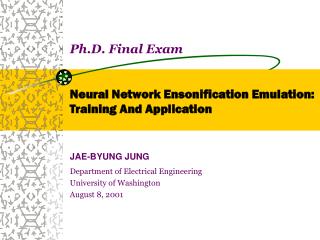
Ph.D. Final Exam Neural Network Ensonification Emulation: Training And Application. JAE-BYUNG JUNG Department of Electrical Engineering University of Washington August 8, 2001. Overview. Review of adaptive sonar Neural network training for varying output nodes On-line training

E N D
Ph.D. Final ExamNeural Network Ensonification Emulation: Training And Application JAE-BYUNG JUNG Department of Electrical Engineering University of Washington August 8, 2001
Overview • Review of adaptive sonar • Neural network training for varying output nodes • On-line training • Batch-mode training • Neural network inversion • Sensitivity analysis • Maximal area coverage problem • Conclusions and ideas for future works
INTRODUCTION- Sonar Surveillance • Software model emulating acoustic propagation • Computationally intensive • Not suitable for real time control Control Sonar Surveillance System Sonar Performance Map Environment
Sonar Data 1 • The physical range-depth output surveillance area is sampled by 30 ranges from 0 to 6 km at steps of 0.2 km and 13 depths from 0 to 200m at steps of 15m • Data Size : 2,500 pattern vectors. (2,000 patterns are used for training the neural network, and 500 patterns are not used for training and reserved for testing.
Sonar Data 2 • The wider surveillance area is considered including 75 sampled ranges from 0 to 15 km at steps of 0.2 km and 20 sampled depths from 0 to 400m at steps of 20m • The shape of SE map varies depending on different bathometry • Data Size : 8,000 pattern vectors. (5,000 patterns are used for training the neural network, and 3,000 patterns are not used for training and reserved for testing)
Neural Network Replacement • Fast Reproduction of SE Map • Inversion (Derivative Existence) • Real-time Control (Optimization)
Training NN • High dimensionality of output space • Multi-Layered Perceptrons • Neural Smithing (e.g. input data jittering, pattern clipping, and weight decay …) • Widely varying bathymetry • Adaptive training strategy for flexible output dimensionality
MLP Training Multilayer perceptrons (MLP’s) typically use a fixed network topology for all training patterns in a data set.
MLP Training with varying output We consider the case where the dimension of the output nodes can vary from training pattern to training pattern
Flexible Dimensionality • Generally, MLP must have a fixed network topology A single neural network can not handle flexible network topology • A modular neural network structure that has local experts for different dimension specific training patterns It becomes increasingly difficult, however, to implement a large number of neural networks as the number of local experts increases
Flexible Dimensionality • Let’s define a new output vector, O, for transformation to fix output dimensionality as where,O(n) is the nth actual output training pattern vector,OA(n) is an arbitrary output vector for O(n) and filled with arbitrary “don’t care” constant numbers • The dimensionality becomes enlarged to be spanned and is fixed as where N is the number of training pattern vectors, Span(·) represents a dimensional span from each output vector to the maximally expandable dimensions over N different pattern vectors, and D(·) represents a dimensionality of the output vector
Flexible Dimensionality • Train a single neural network using a fixed-dimensional output vector O(n) by 1) Filling arbitrary constant value into OA(n) High spatial freq. components are washed out 2) Smearing neighborhood pixels to OA(n) Still need to train unnecessary part (longer training time) • OA(n) can be ignored when O(n) is projected onto O(n) in the testing phase.
Inputs : I(n)={IC(n), IP(n)} IP(n) : profile inputs describe output profile assign each output neuron to either O(n) or OA(n) IC(n) : characteristic inputs contain the other input parameters Outputs : O’(n) ={O(n), OA(n)} OA(n) : “Don’t care” category The weights associated with these neurons are not updated for the nth pattern vector O(n) : Normal weight correction The other weights associated with O(n) are updated with step size modification Don’t Care Training
Advantages Significantly reduced training time by not correcting weights in don’t care category Boundary problem is solved Less training vectors required Focus on active nodes only Drawbacks Rough weight space due to irregular weight correction Possibly leading to local minima Don’t Care Training
Step Size Modification • Even amount of opportunity for weight correction to every output neuron • Statistical information : From the training data set, frequency of weight correction associated with each output neuron are updated.
Step Size Modification • On-line training • Batch-mode training
MSE (Mean Squared Error) MSE can not represent the training performance well due to the different vector size(dimensionality) Average MSE : pixel wise representation of MSE Performance Comparison
Performance Comparison : Training of neural networks
Performance Comparison : Generalization performance from testing error
Contributions:Training • A novel neural network learning algorithm for data sets with varying output node dimension is proposed. • Selective weight update • Fast convergence • Improved accuracy • Step size modification • Good generalization • Improved accuracy
NN Training : Finding Wfrom given input-output relationship NN Inversion : Finding I from given target output T I I W W O O T T Inversion of neural network • W : NN Weight • I : Input • O : Output • T : Target
When we want to find a subset of input vector, i, so that minimize the objective function, E(i), which can be denoted as E(i) = 0.5(ti – oi)2 where oi is the neural network output for input I, and ti is the desired output for input i. If is the kthcomponent of the vector it, then gradient descent suggests the recursion where is the step size and t is the iteration index Iteration for inversion in the equation can be solved as follows Inversion of neural network where, for any neuron,
Single element inversion • The subset of outputs to be inverted is confined in one output pixel at a time during an inversion process while other outputs are floated. • A single input control parameter is achieved during the iterative inversion process while 4 environmental parameters are clamped (fixed) to specific values [wind speed = 7m/s, sound speed at surface = 1500m/s, sound speed at bottom = 1500m/s, and bottom type = 9(soft mud)].
Multiple parameter inversion and maximizing the target area • Multiple output SE values can be inverted at a time • The output target area is tiled with 2x2 pixel regions. Thus, 2x2 output pixel groups are inverted one at a time to find out the best combination of these 5 input parameters to satisfy the corresponding SE values
Pre-Clustering for NN Inversion Pre-clustering of data set from the output space Separate training of partitioned data sets (Local Experts) Training Improvement Inversion Improvement
UnsupervisedClustering Partitioning a collection of data points into a number of subgroups • When we know the number of prototypes • K-NN, Fuzzy C-Means, … • When no a priori information is available. • ART, Kohonen SOFM, …
Adaptive Resonance Theory • Unsupervised learning network developed by Carpenter and Grossberg in 1987 • ART1 is designed for clustering binary vectors • ART2 accepts continuous-valued vectors • F1 layer is an input processing field comprising the input portion and the interface portion. • F2 layer is a cluster unit that is a competitive layer in that the units compete in a winner-take-all mode for the right to learn each input pattern. • The third layer is a reset mechanism that controls the degree of similarity of patterns placed on the same cluster
Training Phase Entire Data Set : Unsupervised Learning ART2 sub-data sub-data sub-data (cluster K) (cluster 1) (cluster 2) Training Training Training : Supervised Learning ANN K ANN 1 ANN 2
Inversion Phase ART2 Cluster 1 (N-Dimension) ART2 Cluster 3 (N-Dimension) ART2 Cluster K (N-Dimension) Desired Output (M-Dimension) Cluster Selection (Projection) ANN 1 Inversion ANN 2 Inversion ANN K Inversion Optimal Input Parameters
Inversion from ART2 Modular Local Experts • Multiple parameter inversion and maximizing the target area. • The output target area is tiled with 2x2 pixel regions. Thus, 2x2 output pixel groups are inverted one at a time to find out the best combination of these 5 input parameters to satisfy the corresponding SE values.
Contributions:Inversion • A new neural network inversion algorithm was proposed whereby several neural networks are inverted in parallel. • Advantages include the ability to segment the problem into multiple sub-problems which each can be independently modified as changes to the system occur over time. • The concept is similar to the mixture of experts problem applied to neural network inversion.
Sensitivity Analysis • Feature selection as neural network is being trained or after the training. Useful to eliminate superfluous input parameters [Rambhia]. • reducing the dimension of the decision space and • increasing speed and accuracy of the system. • When implemented in hardware, the non-linearity occuring in the operation of various network component may practically make a network impossible to train significantly [Jiao]. • very important in the investigation of non-ideal effects. (important issue from the view point of engineering). • Once neural network is trained, it is very important to determine which of the control parameters are critical to the decision making at a certain operating point.
The neural network sensitivity shows how sensitively the output OT responds with respect to the change of the input parameter k. NN Sensitivity ODC (Don’t Care Area) ik OT (Target Surveillance Area)
NN Sensitivity • Chain rule is used to derive where h represents hidden neurons. Generally, for n hidden layers where hn represents neurons in nth hidden layer.
Inversion Sensitivity … neti oi … -1 neti oi ei Inversion vs. Sensitivity ti
NN Sensitivity – output neuron 1. Output Layers : find local gradient of oi at output neuron i neti oi hj wij i
NN Sensitivity – hidden neuron 2. Hidden Layers : find gradient at hidden neuron j with respect to OT netj hj wji i j(netj) j
ik j wkj k NN Sensitivity – input neuron 3. Input Layer : find gradient of OT at input neuron k
Absolute Sensitivity Relative(Logarithmic) Sensitivity Nonlinear Sensitivity
Contributions: Sensitivity Analysis • Once neural network is trained, especially, it is very important to determine which of the control parameters are critical to the decision making at a certain operating point such that environmental situation or/and control criteria is given.
Multiple Objects Optimization • Optimization of multiple objects in order to satisfy system’s maximum cooperating performance. • The composite effort of the system team is significantly more important than a single system’s individual performance
Target Covering Problem • Multiple rectangular boxes move to cover the circular target area. • Each box is situated by 4 parameters including 2 position variables, (x0, y0), an orientation, , and an aspect ratio, r. • The area of each box is fixed.
Target Parameters where (c1, c2) is center of gravity and R is radius of circular target.
Aggregation & Evaluation Aggregation of N boxes : Evaluation of Coverage :