Linear Programming
Linear Programming. Problem Formulation. References. Anderson, Sweeney, Williams: “An Introduction to Management Science, 10th Ed. ”; Thomson Asia Pte. Ltd. Tulsian and Pandey, “Quantitative Techniques – Theory and Problems”; Pearson Education.

Linear Programming
E N D
Presentation Transcript
Linear Programming Problem Formulation
References • Anderson, Sweeney, Williams: “An Introduction to Management Science, 10th Ed.”; Thomson Asia Pte. Ltd. • Tulsian and Pandey, “Quantitative Techniques – Theory and Problems”; Pearson Education The second reference has numerous examples which could be used for self practice.
The three components of a decision making problem • Definition of the decision variables of the problem • Identification of the constraints under which the decision is to be made • Constructing the objective function to be optimized – maximizing contribution to profit or minimizing costs
General Format of a Model Maximize or minimize Objective Function Subject to: Constraints And non-negativity of decision variables Values of the decision variables that satisfy all the constraints including non-negativity, constitute a feasible solution. If the feasible solution maximizes the contribution or minimizes the cost it is an optimum feasible solution.
Linear Programming (LP) • LP applies to optimization models in which the objective and constraint functions are linear • Linearity implies: proportionality + additivity • Proportionality: the contribution of each decision variable in the objective function is proportional to its value. So are the requirements in the constraints • Additivity: the total contribution of the variables in the objective function is the sum of individual contributions of each. So are the requirements in the constraints.
Linear and Programming • Mathematically, a linear function is one in which each variable appears as a separate term and is raised to the first power • The word programming means “choosing a course of action”, i.e. planning activities in a manner that achieves some optimal result within the constraints of resources
Problem Formulation • Problem formulation or modeling is the process of translating the verbal statement of a problem into a mathematical statement. • Formulating models is an art that can only be mastered with practice and experience • The accuracy and value of the conclusions arrived at depends on how well a model represents the real situation
Formulation of an LPP • Identify the Decision Variables of interest to the decision maker and express them as x1, x2, x3, … • Ascertain the Objective of the decision maker • Ascertain the Cost (in case of minimization) or the Profit (in case of maximization) per unit of each decision variable • On the basis of the above data, write down the Objective Function, Z, as a linear function of the decision variables
LPP Formulation (contd.) • Ascertain the Constraints representing the maximum availability (of resources) or the minimum commitment (demands, targets etc.) or equality • Write the constraints in terms of decision variables as “less than or equal to” (<=) type inequality or “greater than or equal to” (>=) type inequality or “equal to” (=) type equality; all constraints shall be linear • Note that maximum availability leads to a <= type and minimum commitment gives a >= type inequality
Formulation (contd.) • Add non-negativity restriction as under: xj >= 0; j = 1, 2, … n Non-negativity constraints are a general feature of all LPPs
The Mathematical Formulation The Mathematical Formulation looks like: Maximize (or Minimize) Z = c1x1 + c2x2 + … Subject to constraints: a11x1 + a12x2+ … <= b1 (Maximum availability) a21x1 + a22x2+ … >= b2 (Minimum commitment) a31x1 + a32x2+ … = b3 (Equality) … x1, x2, … >= 0 (Non-negativity restriction)
A wide range of LP Problems • “Product Mix” Problems (e.g. 1, 2, 3) • “Make or Buy Decision” Problems (e.g. 4) • “Choice of Alternatives” Problems • “Sales Budget” Problems • “Production Budget” Problems • “Purchase Budget” Problems • “Portfolio Mix” Problems (e.g. 5) • “Advertising” Problem
Range of LP Problems (contd.) • “Capital Mix” Problems • “Diet” Problems • Nutrition” Problems • “Blending” Problems • “Trim” Problems • “Transportation” Problems • “Assignment Problems” • “Job Scheduling” Problems
Example 1 A garment manufacturer has a production line making two styles of shirts. Style I needs 200 g of cotton thread, 300 g of dacron thread and 300 g of linen thread. Corresponding requirements of style II are 200g, 200g and 100g. The net contributions are Rs. 19.50 for style I and Rs. 15.90 for style II. The available inventory of cotton thread, dacron thread and linen thread are, respectively, 24 kg, 26 kg and 22 kg. The manufacturer wants to determine the number of each style to be produced with the given inventory. Formulate the LPP model.
Step 1: Objective Function • Decision variables: These are the numbers of each style to be produced: • Number of style I shirts, say x1 • Number of style II shirts, say x2 • Objective of the decision maker: Maximise total contribution, given that the contribution per unit is Rs. 19,50 for x1 and Rs. 15.90 for x2 • Hence the objective function is: Max: Z = 19.50 x1 + 15.90 x2
Step 2: Constraints • Availability of cotton thread: Style I needs 200 g and style II needs 200 g. 24,000 g is available. The corresponding constraint is 200 x1 + 200 x2 <= 24,000 • Availability of dracon thread: Style I needs 300 g and style II needs 200 g. 26,000 g is available. The corresponding constraint is 300 x1 + 200 x2 <= 26,000 • Availability of linen thread: Style I needs 300 g and style II needs 100 g. 22,000 g is available. The corresponding constraint is 300 x1 + 100 x2 <= 22,000
Step 3: Non-negativity Since the number of shirts cannot be negative, add the non-negativity restriction x1, x2 >= 0 and complete the LP formulation. -------------------------------------------------------------- Note: For the time being we ignore another restriction on x1 and x2 that they be integers. If that restriction is also added we write: x1, x2 >=0 and integers. Then this becomes an Integer LP or ILP, which we will see later.
Solution of Example 1 Let x1 = number of style I shirts x2 = number of style II shirts Max: Z = 19.50 x1 + 15.90 x2 (contribution) s.t 200 x1 + 200 x2 <= 24,000 (cotton) 300 x1 + 200 x2 <= 26,000 (dacron) 300 x1 + 100 x2 <= 22,000 (linen) x1, x2 >= 0 (non-negativity)
Example 2 An animal feed company must produce 200 kg of a mixture consisting of ingredients A and B daily. A costs Rs. 3 per kg and B costs Rs. 8 per kg. Not more than 80 kg of A can be used and at least 60 kg of B must be used. The company wants to know how much of each ingredient should be used to minimize cost. Formulate the LPP.
Step 1: Objective Function • Decision variables: Qty of each ingredient used: • Quantity of ingredient A, say A kg • Quantity of ingredient B, say B kg • Objective of the decision maker: Minimise cost, given that cost per unit is Rs. 3 for A; Rs. 8 for B. • Hence the objective function is: Min: Z = 3A + 8B
Step 2: Constraints • Committed output is 200 kg of the mixture. The corresponding constraint is A + B = 200 • Not more than 80 kg of A can be used. The corresponding constraint is A <= 80 • At least 60 kg of B must be used. The corresponding constraint is B >= 60
Step 3: Non-negativity Since the decision variables cannot be negative, add the non-negativity restriction A, B >= 0 and complete the LP formulation. ------------------------------------------------------ Note that we do not have any integer restrictions on the decision variables in this case.
Solution to Example 2 Min: Z = 3A + 8B s.t A + B = 200 A <= 80 B >= 60 A, B >= 0
Example 3 A farmer has a 125 acre farm. He produces radish, mutter and potato. Whatever he raises is fully sold. He gets Rs. 5 per kg for radish, Rs. 4 per kg for mutter and Rs. 5 per kg for potato. The average yield per acre is 1500 kg for radish, 1800 kg for mutter and 1200 kg for potato.Cost of manure per acre is Rs. 187.50, Rs. 225 and Rs. 187.50 for radish, mutter and potato respectively. Labour required per acre is 6 mandays each for radish and potato and 5 man days for mutter. A total of 500 mandays of labour is available at the rate of Rs. 40 per manday. Formulate this as an LPP model to maximise the profit.
Step 1: Objective Function • Decision variables: acreage for each produce: • Acres for radish, say r • Acres for mutter, say m • Acres for potato, say p • Objective of the decision maker: Maximise profit, given that, profit per acre is: • (5*1500 -187.5 – 6*40) for radish • (4*1800 – 225 - 5*40) for mutter • (5*1200 – 187.5 – 6*40) for potato
E.g.: Profit per acre for Radish • Earning per acre Each acre yields 1500 kg. Each kg sells for Rs. 5. Hence earning per acre = Rs. 1500*5 • Cost per acre Manure = Rs. 187.50 Labour = 6 mandays @ Rs, 40 per manday. Hence cost per acre is Rs. (187.50 + 6*40) • Profit = Earning – cost = Rs. (1500*5 – 187.5 – 6*40)
Step 2: Constraints • Availability of land = 125 acres. The corresponding constraint is r + m + p <= 125 • Availability of labour = 500 mandays. The corresponding constraint is 6r + 5m + 6p <= 500
Step 3: Non-negativity Since the decision variables cannot be negative, add the non-negativity restriction r, m, p >= 0 and complete the LP formulation.
Solution to Example 3 Let r, m, p be the no of acres used for radish, mutter and potato respectively. Max (5*1500 -187.5 – 6*40) r + (4*1800 – 225 - 5*40) m + (5*1200 – 187.5 – 6*40)p s.t r + m + p <= 125 (Land constraint) 6r + 5m + 6 p <= 500 (Mandays constraint) r, m, p >= 0 (non-negativity)
Example 4 Jindal manufactures a type of sofa set containing seven components: one sofa, two centre tables and four chairs. These can either be manufactured in-house or sub-contracted as per the data given in the table: Sales of sofa sets are 8,000 per period, each selling for Rs.7,500. A capacity constraint of 500,000 direct labour hours obliges the company to sub-contract some components. The variable overheads vary with direct labour hours at Rs. 2 per hour. Fixed costs are Rs. 1,750,000 per period and labour costs Rs. 5.50 per hour. Formulate LPP to minimise costs.
Decision variables: The nos of sofas, tables, chairs made / bought: sm, sb, tm, tb, cm, cb. • The table on the next slide calculates the cost per unit of each decision variable (objective function coefficients) • Hence the objective function is: Min 1750 sm +2500 sb + 875 tm + 1000 tb + 625 cm + 750 cb • Constraints: • Demand for sofas: sm + sb = 8000 • Demand for tables: tm + tb = 16,000 • Demand for chairs: cm + cb = 32,000 • Direct labour hours: 100 sm + 50 tm + 10 cm <= 500,000 • Non-negativity: sm, sb, tm, tb, cm, cb >= 0
Solution to example 4 Minimise 1750 sm + 2500 sb + 875 tm + 1000 tb + 625 cm + 750 cb Subject to: sm + sb = 8000 (demand for sofas) tm + tb = 16,000 (demand for table) cm + cb = 32,000 (demand for chairs) 100 sm + 50 tm + 10 cm <= 500,000 (direct labour available) sm, sb, tm, tb, cm, cb >= 0 (non-negativity)
Example 5 A mutual fund has Rs. 2 million available for investment in Government bonds, blue chip stocks, speculative stocks and short-term bank deposits. The annual expected return and the risk factor are as shown: The fund is required to keep at least Rs. 200,000 in short-term deposits and not to exceed an average risk factor of 42. Speculative stocks must not exceed 20% of the money invested. Formulate the LPP maximizing expected annual return.
Decision variables: Amounts invested in Government bonds, blue chip stocks, speculative stocks and short-term bank deposits : x1, x2, x3 and x4. • Objective: Maximise returns given that the return per Re. for the investments are 0.14, 0.19, 0.23, 0.12 • Hence the objective function is: Max 0.14 x1 + 0.19 x2 + 0.23 x3 + 0.12 x4 • Constraints: (See next slide for calculations) • Amount available: x1 + x2 + x3 + x4.<= 2,000,000 • At least 200,000 in STD: x4 >= 200,000 • Average risk factor: 30x1+18x2-6x3+36x40 • Limit on speculative stock: 0.2 x1 + 0.2 x2 – 0.8 x3 + 0.2 x4 0 • Non-negativity: x1, x2, x3, x4 >= 0
Solution to Example 5 Let x1, x2, x3, x4 be the amounts invested. Average risk factor = (12 x1+24 x2 + 48 x3 + 6 x4)/(x1+ x2+ x3+ x4) 42. This gives 30x1+18x2-6x3+36x40. Also x3 0.2 (x1+ x2+ x3+ x4) ---- Maximum limit on speculative stock This gives: 0.2 x1 + 0.2 x2 – 0.8 x3 + 0.2 x4 0 Hence the LPP formulation is as follows: Max: 0.14 x1+ 0.19 x2+ 0.23 x3+ 0.12 x4 s.t: 30x1+18x2-6x3+36x40 (Avg Risk factor) 0.2 x1 + 0.2 x2 – 0.8 x3 + 0.2 x4 0 (limit on speculative stock) x1 + x2+ x3 + x4 2,000,000 x4 200,000 x1, x2, x3, x4 0 (Non-negativity)
Example 6 The vitamins V and W are found in two different foods, F1 and F2. The respective prices per unit of each food are Rs. 3 and Rs. 2.5. One unit of F1 contains 2 units of vitamin V and 3 units of vitamin W. One unit of F2 contains 4 units of vitamin V and 2 units of vitamin W. The daily requirements of V and W are at least 60 units and 75 units respectively. Formulate an LPP to meet the daily requirement of the vitamins at minimum cost
Decision variables: Quantity of foods F1 and F2 required be x1 and x2. • Objective: Minimise cost given that the costs per unit of F1 and F2 are Rs. 3 and Rs. 2.5 respectively • Hence the objective function is: Minimise 3 x1 + 2.5 x2 • Constraints: • Requirement of V: 2x1 + 4 x2 60 • Requirement of W: 3x1 + 2 x2 75 • Non-negativity: x1, x2, x3, x4 >= 0
Solution to Example 6 Let x1 and x2 be the quantities of F1 and F2. Minimise: 3x1 + 2.5 x2 s.t: 2x1 + 4 x2 60 (Min requirement of V) 3x1 + 2x2 75 (Min requirement of W) x1 , x2 0

