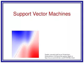
Support Vector Machines
Support Vector Machines. H. Clara Pong Julie Horrocks 1 , Marianne Van den Heuvel 2 ,Francis Tekpetey 3, B. Anne Croy 4. 1 Mathematics & Statistics, University of Guelph, 2 Biomedical Sciences, University of Guelph, 3 Obstetrics and Gynecology, University of Western Ontario,

Support Vector Machines
E N D
Presentation Transcript
Support Vector Machines H. Clara Pong Julie Horrocks1, Marianne Van den Heuvel2,Francis Tekpetey3, B. Anne Croy4. 1 Mathematics & Statistics, University of Guelph, 2 Biomedical Sciences, University of Guelph, 3 Obstetrics and Gynecology, University of Western Ontario, 4 Anatomy & Cell Biology, Queen’s University
Outline • Background • Separating Hyper-plane & Basis Expansion • Support Vector Machines • Simulations • Remarks
CD56 bright cells Background • Motivation • The IVF (In-Vitro Fertilization) project • 18 infertile women • each undergoing the IVF treatment • Outcome (Outputs, Y’s) : Binary (pregnancy) • Predictor (Inputs, X’s): Longitudinal data (adhesion)
Background • Classification methods • Relatively new method: Support Vector Machines • V. Vapnik: first proposed in 1979 • Maps input space into a high dimensional feature space • Constructs a linear classifier in the new feature space • Traditional method: Discriminant Analysis • R.A. Fisher: 1936 • Classify according to the values from the discriminant functions • Assumption: the predictors X in a given class has a Multi-Normal distribution.
f(X) = β0 +βTX =0 A: f(X)>0 B: f(X)<0 Separating Hyper-plane Suppose there are 2 classes (A, B) • y = 1 for group A, y = -1 for group B. Let a hyper-plane be defined as f(X) = β0 +βTX = 0 then f(X) is the decision boundary that separates the two groups. f(X) = β0 +βTX > 0 for X Є A f(X) = β0 +βTX < 0 for X Є B Given X0 Є A, misclassified when f(X0 ) < 0. Given X0 Є B , misclassified when f(X0 ) > 0.
f(X) = β0 +βTX =0 Separating Hyper-plane The perceptron learning algorithm search for a hyper-plane that minimizes the distance of misclassified points to the decision boundary. However this does not provide a unique solution.
C C f(X) = β0* +β*TX = 0 Optimal Separating Hyper-plane Let C be the distance of the closest point from the two groups to the hyper-plane. The Optimal Separating hyper-plane is the unique separating hyper-plane f(X) = β0* +β*TX = 0, where (β*0 ,β*T) maximizes C.
Dual LaGrange problem: f(X) = β0* +β*TX = 0 C C (the support vectors) Optimal Separating Hyper-plane Maximization Problem: Subjects to 1. αi [yi (xiTβ+ β0) -1] = 0 2. αi ≥ 0 all i=1…N 3. β = Σi=1..Nαi yixi 4. Σi=1..Nαi yi = 0 5. The Kuhn Tucker Conditions f(X) only depends on the xi’s where αi ≠ 0
f(X) = β0* +β*TX = 0 C C (the support vectors) Optimal Separating Hyper-plane
x1x2 x2 + x2 x1 x1 + Basis Expansion Suppose there are p inputs X=(x1 … xp) Let hk(X) be a transformation that maps X from RpR. hk(X) is called the basis function. H = {h1(X), … ,hm(X)} is the basis of a new feature space (dim=m) Example: X=(x1,x2) H = {h1(X), h2(X),h3(X)} h1(X) = h1(x1,x2) = x1, h2(X) = h2(x1,x2) =x2, h3(X) = h3(x1,x2) =x1x2 X_new = H(X)= (x1, x2, x1x2)
Separable Case:all points are outside of the margins The classification rule is the sign of the decision function. C C f(X) = β0* +β*TX = 0 Support Vector Machines The optimal hyper-plane {X| f(X) = β0* +β*TX=0 }. f(X) = β0* +β*TX is called the Support Vector Classifier.
yif(Xi) C Si Support Vector Machines Non-separable Case:training data is non-separable. Hyper-plane: {X| f(X) = β0 +βTX = 0 } f(X) = β0 +βTX = 0 Xi crosses the margin of its group when C – yi f(Xi) > 0. Si = C – yi f(Xi) when Xi crosses the margin and it’s zero when Xi outside. LetξiC =Si, ξi is the proportional of C that the prediction has crossed the margin. Misclassification occurs when Si > C (ξi > 1).
Maximization Problem: Dual LaGrange problem: (non-separable case) s.t. . 0≤ αi ≤ ζ , Σ αi yi = 0 Subjects to 1. αi [yi (xiTβ+ β0) –(1-ξi)] = 0 2. vi ≥ 0 all i=1…N 3. β = Σ αiyixi 4. The Kuhn Tucker Conditions Support Vector Machines The overall misclassification is Σξi , and is bounded by δ.
The linear classifier becomes Dual LaGrange problem: Support Vector Machines SVM search for an optimal hyper-plane in a new feature space where the data are more separate. Suppose H = {h1(X), … ,hm(X)} is the basis for the new feature space F. All elements in the new feature space is a linear basis expansion of X.
Kernel: For example: This implies Support Vector Machines The kernel and the basis transformation define one another.
The most common kernels: 1. dth Degree Polynomial: 2. Radial Basis: 3. Neural Network: Support Vector Machines Dual LaGrange function: This shows the basis transformation in SVM does not need to be define explicitly.
Simulations • 3 cases • 100 simulations per case • Each simulation consists of 200 points • 100 points from each group • Input space: 2 dimensional • Output: 0 or 1 (2 groups) • Half of the points are randomly selected as the training set. X=(x1,x2), Y є {0,1}
Black ~ group 0 Red ~ group 1 Simulations Case 1 (Normal with same covariance matrix)
Simulations Case 1
Black ~ group 0 Red ~ group 1 Simulations Case 2 (Normal with unequal covariance matrixes)
Simulations Case 2
Black ~ group 0 Red ~ group 1 Simulations Case 3 (Non-normal)
Simulations Case 3
Simulations Paired t-test for differences in misclassifications Ho: mean different = 0; Ha: mean different ≠ 0 Case 1 mean different (LDA - SVM) = - 0.41 , se = 0.3877 t = -1.057, p-value = 0.29 (insignificant) Case 2 mean different (QDA - SVM) = -1.96 , se = 0.4170 t = -4.70, p-value = 8.42e-06 (significant) Case 3 mean different (QDA - SVM) = 2, sd= 0.4218 t = 4.74, p-value = 7.13e-06 (significant)
Remarks Support Vector Machines • Maps the original input space onto a feature space of higher dimension • No assumption on the distributions of X’s Performance • The performances of Discriminant Analysis and SVM are similar (when (X|Y) has a Normal distribution and share the same Σ) • Discriminant Analysis has a better performance (when the covariance matrices for the two groups are different) • SVM has a better performance (when the input (X) violated the distribution assumption)
Reference • N. Cristianini, and J. Shawe-Taylor An introduction to Support Vector Machines and other kernel-based learning methods. New York: Cambridge University Press, 2000. • J. Friedman, T. Hastie, and R. Tibshirani The Elements of Statistical Learning. NewYork: Springer, 2001. • D. Meyer, C. Chang, and C. Lin.R Documentation: Support Vector Machines.http://www.maths.lth.se/help/R/.R/library/e1071/html/svm.html Last updated: March 2006 • H. Planatscher and J. Dietzsch. SVM-Tutorial using R (e1071-package) http://www.potschi.de/svmtut/svmtut.htm • M. Van Den Heuvel, J. Horrocks, S. Bashar, S. Taylor, S. Burke, K. Hatta, E. Lewis, and A. Croy. Menstrual Cycle Hormones Induce Changes in Functional Interac-tions Between Lymphocytes and Endothelial Cells. Journal of Clinical Endocrinology and Metabolism, 2005.