Mathematical Modeling Techniques for Analyzing Relationships Between Data and Equations
Explore various mathematical modeling approaches such as neural networks, Bayesian statistics, cellular automata, simulated annealing, evolutionary algorithms, and parameter optimization for fitting models to data. Learn techniques for developing functional or mechanistic models, based on the complexity of the system and data availability. Discover how to express relationships mathematically, obtain parameter values, and analyze them using statistical software.


Mathematical Modeling Techniques for Analyzing Relationships Between Data and Equations
E N D
Presentation Transcript
Step 5) Express the relationships mathematically in equations Step 6) Get values of parameters Determine what type of model you will make - functional or mechanistic Use ”standard” equations if possible Analyse relationships with a statistical software
Which techniques should be used to develop your mathematical model? Potential candidate equations known Known Unknown Form of Equation Not complex Complex Not complex Complexity of system Extensive Limited Extensive Limited Availability of data Statistical fitting Bayesian statistics Cellular automata Simulated annealing Evolutionary algorithm Neural networks Parameter optimisation
Form of equation: unknown. System: not complex. Data: Extensive Neural networks Input nodes ar set up, analogous to the neural nodes in the brain Through a iterative ”training” process different weights are given to the different connections in the network http://www.oup.com/uk/orc/bin/9780199272068/01student/weblinks/ch02/smith_smith_box2b.pdf
Potential candidated equations known Bayesian statistics (or Bayesian inference) Estimates the probability of different hypothesis (candidate models) instead of rejection of hypothesis which is the more common approach http://www.oup.com/uk/orc/bin/9780199272068/01student/weblinks/ch02/smith_smith_box2c.pdf
Form of equation: known. System: complex but can be simplified. Data: Limited Cellular automata For processes that have a spatial dimension (2D or 3D) Equations for the interaction between neighboring cells are fitted http://www.oup.com/uk/orc/bin/9780199272068/01student/weblinks/ch02/smith_smith_box2e.pdf
Form of equation: known. System: complex. Data: Extensive Simulated annealing Simulated annealing: used to locate a good approximation to the global optimum of a given function in a large search space The process is iterated until a satisfactory level of accuracy is achieved. http://www.oup.com/uk/orc/bin/9780199272068/01student/weblinks/ch02/smith_smith_box2f.pdf
Form of equation: known. System: complex. Data: Extensive Evolutionary algorithm Evolutionary algorithms: are similar to what is used in simulated annealing, but instead of mutating parameter values the rules themselves are altered. Fitness of the rule set is measured in terms of both how well the model fits the data, and how complex the model is. A simple model, which gives the same results as a complex one is preferable. http://www.oup.com/uk/orc/bin/9780199272068/01student/weblinks/ch02/smith_smith_box2f.pdf
Form of equation: known. System: not complex Parameter optimisation of known equations Form of equation: unknown. System: not complex Statistical fitting Example of curve fitting tools Excel - Only functions that can be solved analytically with least square methods Statistical software, e.g. SPSS Matlab Special curve fitting tools, e.g. TabelCurve
Additive or multiplicative functions Additive Y = f(A) + f(B) Y 0-1 If equal weight: f(A) 0-0.5, f(B) 0-0.5 If f(A) = 0 and f(B) = 0 then y = 0 If f(A) = 0 and f(B) = 0.5 then y = 0.5 If f(A) = 0.5 and f(B) = 0 then y = 0.5 If f(A) = 0.5 and f(B) = 0.5 then y = 1 Multiplicative Y = f(A) × f(B) Y 0-1 If equal weight: f(A) 0-1, f(B) 0-1 If f(A) = 0 and f(B) = 0 then y = 0 If f(A) = 0 and f(B) = 1then y = 0 If f(A) = 1 and f(B) = 0 then y = 0 If f(A) = 1 and f(B) = 1 then y = 1
Example - stepwise fitting of a multiplicative function Model of transpiration Lagergren and Lindroth 2002
Example - stepwise fitting of a multiplicative function First try to find a theorethical base for the model (r) (DVPD) (θ) (T) Lagergren and Lindroth 2002
Example - stepwise fitting of a multiplicative function Envelope fitting of the first dependency (Alternately: Select a period when you expect no limitation from r, T or θ) Gives: gmax and f(DVPD)
Example - stepwise fitting of a multiplicative function Select a period when you expect no limitation from T or θ
Example - stepwise fitting of a multiplicative function Select a period when you expect no limitation from θ
Example - stepwise fitting of a multiplicative function The remaining deviation should be explained by θ
Example - stepwise fitting of a multiplicative function The modelled was controlled by applying it for the callibration year And validated against a different year