Conditional Probability Distributions
Conditional Probability Distributions. Eran Segal Weizmann Institute. Last Time. Local Markov assumptions – basic BN independencies d-separation – all independencies via graph structure G is an I-Map of P if and only if P factorizes over G

Conditional Probability Distributions
E N D
Presentation Transcript
Conditional Probability Distributions Eran Segal Weizmann Institute
Last Time • Local Markov assumptions – basic BN independencies • d-separation – all independencies via graph structure • G is an I-Map of P if and only if P factorizes over G • I-equivalence – graphs with identical independencies • Minimal I-Map • All distributions have I-Maps (sometimes more than one) • Minimal I-Map does not capture all independencies in P • Perfect Map – not every distribution P has one • PDAGs • Compact representation of I-equivalence graphs • Algorithm for finding PDAGs
CPDs • Thus far we ignored the representation of CPDs • Today we will cover the range of CPD representations • Discrete • Continuous • Sparse • Deterministic • Linear
Table CPDs • Entry for each joint assignment of X and Pa(X) • For each pax: • Most general representation • Represents every discrete CPD • Limitations • Cannot model continuous RVs • Number of parameters exponential in |Pa(X)| • Cannot model large in-degree dependencies • Ignores structure within the CPD I S P(I) P(S|I)
Structured CPDs • Key idea: reduce parameters by modeling P(X|PaX) without explicitly modeling all entries of the joint • Lose expressive power (cannot represent every CPD)
Deterministic CPDs • There is a function f: Val(PaX) Val(X) such that • Examples • OR, AND, NAND functions • Z = Y+X (continuous variables)
Deterministic CPDs • Replace spurious dependencies with deterministic CPDs • Need to make sure that deterministic CPD is compactly stored T1 T2 T1 T2 T S S
Ind(S1;S2 | T1,T2) Deterministic CPDs • Induce additional conditional independencies • Example: T is any deterministic function of T1,T2 T1 T2 T S2 S1
Ind(D;E | B,C) Deterministic CPDs • Induce additional conditional independencies • Example: C is an XOR deterministic function of A,B D A B C E
Ind(S1;S2 | T1=t1) Deterministic CPDs • Induce additional conditional independencies • Example: T is an OR deterministic function of T1,T2 T1 T2 T S2 S1 Context specific independencies
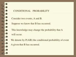
Context Specific Independencies • Let X,Y,Z be pairwise disjoint RV sets • Let C be a set of variables and cVal(C) • X and Y are contextually independentgiven Z and c, denoted (XcY | Z,c) if:
A B C D A a0 a1 (0.2,0.8) B b0 b1 C (0.4,0.6) c0 c1 (0.9,0.1) (0.7,0.3) 4 parameters Tree CPDs A B C D 8 parameters
State 1 State 2 State 3 Repressor Regulated gene Activator Activator Activator Activator Repressor Activator Repressor Repressor Regulators Regulators DNA Microarray DNA Microarray Regulated gene Regulated gene Regulated gene Gene Regulation: Simple Example
Regulation program Module genes Regulation Tree Segal et al., Nature Genetics ’03 Activator? Activator expression false true true Repressor? Repressor expression false true State 1 State 2 State 3
Regulation program Module genes Respiration Module Segal et al., Nature Genetics ’03 • Module genes known targets of predicted regulators? Predicted regulator Hap4+Msn4 known to regulate module genes
Rule CPDs • A rule r is a pair (c;p) where c is an assignment to a subset of variables C and p[0,1]. Let Scope[r]=C • A rule-based CPD P(X|Pa(X)) is a set of rules R s.t. • For each rule rR Scope[r]{X}Pa(X) • For each assignment (x,u) to {X}Pa(X) we have exactly one rule (c;p)R such that c is compatible with (x,u).Then, we have P(X=x | Pa(X)=u) = p
Rule CPDs • Example • Let X be a variable with Pa(X) = {A,B,C} • r1: (a1, b1, x0; 0.1) • r2: (a0, c1, x0; 0.2) • r3: (b0, c0, x0; 0.3) • r4: (a1, b0, c1, x0; 0.4) • r5: (a0, b1, c0; 0.5) • r6: (a1, b1, x1; 0.9) • r7: (a0, c1, x1; 0.8) • r8: (b0, c0, x1; 0.7) • r9: (a1, b0, c1, x1; 0.6) • Note: each assignment maps to exactly one rule • Rules cannot always be represented compactly within tree CPDs
Tree CPDs and Rule CPDs • Can represent every discrete function • Can be easily learned and dealt with in inference • But, some functions are not represented compactly • XOR in tree CPDs: cannot split in one step on a0,b1 and a1,b0 • Alternative representations exist • Complex logical rules
A=a1 Ind(D,C | A=a1) A B C D A=a0 Ind(D,B | A=a0) A B C D Context Specific Independencies A B C D A a0 a1 C B c0 c1 b0 b1 (0.9,0.1) (0.7,0.3) (0.2,0.8) (0.4,0.6) Reasoning by cases implies that Ind(B,C | A,D)
Independence of Causal Influence • Causes: X1,…Xn • Effect: Y • General case: Y has a complex dependency on X1,…Xn • Common case • Each Xi influences Y separately • Influence of X1,…Xn is combined to an overall influence on Y ... X1 X2 Xn Y
Example 1: Noisy OR • Two independent effects X1, X2 • Y=y1 cannot happen unless one of X1, X2 occurs • P(Y=y0 | X1=x10 , X2=x20) = P(X1=x10)P(X2=x20) X1 X2 Y
Noisy OR: Elaborate Representation X1 X2 X’1 X’2 Noisy CPD 1 Noisy CPD 2 Y Noise parameter X1=0.9 Noise parameter X1=0.8 Deterministic OR
Noisy OR: Elaborate Representation Decomposition results in the same distribution
Noisy OR: General Case • Y is a binary variable with k binary parents X1,...Xn • CPD P(Y | X1,...Xn) is a noisy OR if there are k+1 noise parameters 0,1,...,nsuch that
Noisy OR Independencies X1 X2 Xn ... X’1 X’2 X’n Y ij: Ind(Xi Xj | Y=yo)
Generalized Linear Models • Model is a soft version of a linear threshold function • Example: logistic function • Binary variables X1,...Xn,Y
General Formulation • Let Y be a random variable with parents X1,...Xn • The CPD P(Y | X1,...Xn) exhibits independence of causal influence (ICI) if it can be described by • The CPD P(Z | Z1,...Zn) is deterministic ... X1 X2 Xn ... Noisy OR Zi has noise model Z is an OR function Y is the identity CPD Logistic Zi = wi1(Xi=1) Z = Zi Y = logit (Z) Z1 Z2 Zn Z Y
General Formulation • Key advantage: O(n) parameters • As stated, not all that useful as any complex CPD can be represented through a complex deterministic CPD
Continuous Variables • One solution: Discretize • Often requires too many value states • Loses domain structure • Other solution: use continuous function for P(X|Pa(X)) • Can combine continuous and discrete variables, resulting in hybrid networks • Inference and learning may become more difficult
0.4 0.35 0.3 0.25 0.2 0.15 0.1 0.05 0 -4 -2 0 2 4 Gaussian Density Functions • Among the most common continuous representations • Univariate case:
Gaussian Density Functions • A multivariate Gaussian distribution over X1,...Xn has • Mean vector • nxn positive definite covariance matrix positive definite: • Joint density function: • i=E[Xi] • ii=Var[Xi] • ij=Cov[Xi,Xj]=E[XiXj]-E[Xi]E[Xj] (ij)
Gaussian Density Functions • Marginal distributions are easy to compute • Independencies can be determined from parameters • If X=X1,...Xn have a joint normal distribution N(;) then Ind(Xi Xj) iff ij=0 • Does not hold in general for non-Gaussian distributions
Linear Gaussian CPDs • Y is a continuous variable with parents X1,...Xn • Y has a linear Gaussian model if it can be described using parameters 0,...,nand 2such that • Vector notation: • Pros • Simple • Captures many interesting dependencies • Cons • Fixed variance (variance cannot depend on parents values)
Linear Gaussian Bayesian Network • A linear Gaussian Bayesian network is a Bayesian network where • All variables are continuous • All of the CPDs are linear Gaussians • Key result: linear Gaussian models are equivalent to multivariate Gaussian density functions
Linear Gaussian BNs define a joint Gaussian distribution Equivalence Theorem • Y is a linear Gaussian of its parents X1,...Xn: • Assume that X1,...Xn are jointly Gaussian with N(;) • Then: • The marginal distribution of Y is Gaussian with N(Y;Y2) • The joint distribution over {X,Y} is Gaussian where
Converse Equivalence Theorem • If {X,Y} have a joint Gaussian distribution then • Implications of equivalence • Joint distribution has compact representation: O(n2) • We can easily transform back and forth between Gaussian distributions and linear Gaussian Bayesian networks • Representations may differ in parameters • Example: • Gaussian distribution has full covariance matrix • Linear Gaussian ... X1 X2 Xn
Hybrid Models • Models of continuous and discrete variables • Continuous variables with discrete parents • Discrete variables with continuous parents • Conditional Linear Gaussians • Y continuous variable • X = {X1,...,Xn} continuous parents • U = {U1,...,Um} discrete parents • A Conditional Linear Bayesian network is one where • Discrete variables have only discrete parents • Continuous variables have only CLG CPDs
Hybrid Models • Continuous parents for discrete children • Threshold models • Linear sigmoid
Summary: CPD Models • Deterministic functions • Context specific dependencies • Independence of causal influence • Noisy OR • Logistic function • CPDs capture additional domain structure