Chapter 2 Divide-and-Conquer
Chapter 2 Divide-and-Conquer. 2.1 Divide-and-Conquer Approach 2.2 Binary Search 2.3 Mergesort 2.4 Quicksort (Partition Exchange Sort) 2.5 Strassen’s Matrix Multiplication Algorithm 2.6 Arithmetic with Large Integers 2.7 Fast Fourier Transform (FFT) 2.8 Determining Thresholds.

Chapter 2 Divide-and-Conquer
E N D
Presentation Transcript
Chapter 2Divide-and-Conquer 2.1 Divide-and-Conquer Approach 2.2 Binary Search 2.3 Mergesort 2.4 Quicksort (Partition Exchange Sort) 2.5 Strassen’s Matrix Multiplication Algorithm 2.6 Arithmetic with Large Integers 2.7 Fast Fourier Transform (FFT) 2.8 Determining Thresholds Divide-and-Conquer
The divide-and-conquer design strategy involves the following steps: Divide an instance of a problem into one or more smaller instances. Conquer (solve) each of the smaller instances. Unless a smaller instance is sufficiently small, use recursion to do this. If necessary, combine the solutions to the smaller instances to obtain the solution to the original instance. 2.1: Divide-and-Conquer Approach Divide-and-Conquer
Problem: Determine whether x is in the sorted array S of size n. The steps of Binary Search can be summarized as follows: Divide the array into two subarrays about half as large. If x is smaller than the middle term, choose the left subarray; otherwise, choose the right subarray. Conquer (solve) the subarray by determining whether x is in that subarray. Unless the subarray is sufficiently small, use recursion to do this. Obtain the solution to the array from the solution to the subarray. 2.2: Binary Search Divide-and-Conquer
Suppose x = 18 and we have the following array: 10 12 13 14 18 20 25 27 30 35 40 45 47 Divide the array: because x < 25, we need to search 10 12 13 14 18 20 Conquer the subarray by determining whether x is in that subarray recursively. The answer is Yes. Obtain the solution to the array from the solution to the subarray. Yes, x is in that array. Middle term Example 2.1 Divide-and-Conquer
Algorithm 2.1:Binary Search (Recursive) • Problem:Determine whether x is in the sorted array S of size n. Inputs:positive integer n, sorted array of keys S indexed from1 to n, and a key x. Output:location, the location of x in S (0 if x is not in S) • indexlocation(indexlow, indexhigh) {indexmid; if (low >high ) return 0; else{mid = (low + high )/2; if (x= =S[mid]) location = mid; else if(x<S[mid]) returnlocation(low,mid1); elsereturnlocation(mid+1,high); } } Divide-and-Conquer
Compare x with 25 10 12 13 14 18 20 Compare x with 13 14 18 20 Compare x with 18 Because x= 18, xis in S. Recursive Steps of Example 2.1 10 12 13 14 18 20 25 27 30 35 40 45 47 Because x< 25, choose left subarray. Because x> 13, choose right subarray. Divide-and-Conquer
Comparison in recursive call Comparison at top level Analysis of Algorithm 2.1 • Worst-Case Time Complexity By applying Master Theorem, a = 1, b = 2, d = 0, so a = bd Hence, Divide-and-Conquer
2.3 Mergesort • What is Mergesort? 1.Dividethe array into two subarrays each with n/2 items. 2.Conquer (solve) each subarray by sorting it recursively, unless the array is sufficiently small. 3.Combine the solutions to the subarrays by merging them into a single sorted array. Divide-and-Conquer
Example 2.2 Suppose the array contains these numbers in sequence: 27 10 12 20 25 13 15 22 1. Divide the array: 27 10 12 20 and25 13 15 22 2. Sort each array: 10 12 20 27 and13 15 22 25 3. Merge the subarrays: 10 12 13 15 20 22 25 27 Divide-and-Conquer
Algorithms 2.2:Mergesort • Problem:Sort n keys in nondecreasing sequence. Inputs:positive integer n, array of keys S index from 1 to n. Output:the array S containing the keys in nondecreasing sequence. • voidmergesort(intn, keytype S[]) { if ( n > 1) { const inth = n/2 , m = n h; keytype U[1..h] , V[1..m] ; copy S[1] through S[h] to U[1] through U[h]; copy S[h+1] through S[n] to V[1] through V[h]; mergesort(h, U); mergesort(m, V); merge(h, m, U, V, S); } } Divide-and-Conquer
27 10 12 20 25 13 15 22 27 10 12 20 25 13 15 22 25 13 15 22 27 10 12 20 10 27 12 20 13 25 15 22 10 12 20 27 13152225 1012131520222527 Recursive Steps for Example 2.2 27 10 12 20 25 13 15 22 Divide-and-Conquer
Algorithm 2.3:Merge • voidmerge(inth, intm, const keytype U[], const keytype V[], keytypeS[]) { index i, j, k ; i = 1; j = 1; k = 1; while ( i <= h&&j <= m) { if (U[i] < V[j]) { S[k] = U[i]; i++; } else { S[k] = V[j]; j++; } k++; } if (i > h) copy V[j] through V[m] to S[k] through S[h+m]; else copy U[i] through U[h] to S[k] through S[h+m]; } Divide-and-Conquer
Analysis of Algorithm 2.3 • Worst-Case Time Complexity (Merge) Merge U[h] and V[m] to S[h+m] One of the worst-case: S[]={U[1],U[2],…,U[h1],V[1],V[2],…,V[m],U[h]} The number of comparisons of U[i] and V[j]: h+m1 Hence, the worst-case time complexity is W(h,m)=h+m1 Divide-and-Conquer
2 mergersort 1 merge Analysis of Algorithm 2.2 • Worst-Case Time Complexity (Mergesort) Let W(n) be the time complexity to sort S[n]. Divide S[n] into 2subarrays with size n/2, call mergesort for each subarray, and then merge them. W(n) = 2W(n/2) + (n/2+n/21) = 2W(n/2) + n1 Using Master Theorem, a = 2, b = 2, d = 1, so a = bd , W(n) (n log2 n) Divide-and-Conquer
Algorithm 2.4:Mergesort 2 • voidmergesort2 (indexlow, indexhigh) { indexmid; if (low < high) { mid = (low + high)/2 ; mergesort2(low , mid); mergesort2(mid +1 , high); merge2(low, mid, high); } } Divide-and-Conquer
Algorithm 2.5:Merge 2 • voidmerge2(indexlow,indexmid, indexhigh) { indexi, j, k ; keytype U[low..high]; i = low; j = mid + 1; k= low; while (imid&& j high ) { if (S[i] < S[j]) { U[k] = S[i]; i ++; } else { U[k] = S[j]; j ++; } k ++; } if (i > mid) move S[j] through S[high] to U[k] through U[high]; else move S[i] through S[mid] to U[k] through U[high]; move U[low] through U[high] to S[low] through S[high]; } Divide-and-Conquer
Pivot item 15 22 13 27 12 10 20 25 10 15 15 15 10 13 13 13 13 12 13 12 22 12 12 27 15 10 27 15 12 22 20 22 22 22 27 27 10 10 25 20 20 20 20 25 25 25 25 27 2.4 Quicksort (Partition Exchange Sort) Example 2.3 Suppose the array:1522 13 27 12 10 20 25 Partition the array:all items < pivot are to the left and all items> pivot to the right 2.Sort the subarrays: Divide-and-Conquer
Steps of Quicksort Divide-and-Conquer
Algorithm 2.6:Quicksort • Problem:Sort n keys in nondecreasing order. • Inputs:positive integer n, array of keys S index • from 1 to n. • Outputs: the array S containing the keys in • nondecreasing order. • voidquicksort (indexlow, indexhigh) • { indexpivotpoint; • if (high > low) • { partition(low, high, pivotpoint) • quicksort ( low, pivotpoint-1) ; • quicksort (pivotpoint+1, high) • } • } Divide-and-Conquer
15 22 13 27 12 10 20 25 15 10 15 15 13 13 13 13 12 12 12 22 15 27 10 27 12 22 22 22 27 10 10 27 20 20 20 20 25 25 25 25 Algorithm 2.7:Partition voidpartition (indexlow, indexhigh, index& pivotpoint) { indexi, j; keytypepivotitem; pivotitem = S[low]; j = low; for (i = low + 1; i high; i ++) if (S[i] < pivotitem) { j ++; exchange S[i] and S[j]; } pivotpoint = j; exchange S[low] and S[pivotpoint]; } Divide-and-Conquer
Steps of Partition Divide-and-Conquer
Analysis of Algorithm 2.7 (Partition) • Every-Case Time Complexity (Partition) Basic operation:the comparison of S[i] with pivotitem. Input size: n = high low+1, the number of items in the subarray. Every item except the first is compared. Hence, T(n) = n-1. Divide-and-Conquer
Time to sort right subarray Time to sort left subarray Time to partition Analysis of Algorithm 2.6 • Worst-Case Time Complexity (Quicksort) W(n) = W(0) + W(n1) +n1 = W(n1) +n1 = n(n1)/2 W(n) (n2) Divide-and-Conquer
Average time to sort subarrays when pivotpoint is p Time to partition Analysis of Algorithm 2.6 • Average-Case Time Complexity Divide-and-Conquer
15 22 13 27 12 10 20 25 15 15 10 10 13 10 13 12 13 15 12 27 12 27 27 22 22 22 20 20 20 25 25 25 Another Partition Method voidpartition2 (indexlow, indexhigh, index& pivotpoint) { indexi, j; keytypepivotitem; pivotitem = S[low]; i = low; j = high+1; while (i< j) {while (i < high && S[i+1] < pivotitem) i++; while (j > low &&S[j1] > pivotitem) j; i++;j; if (i < j) exchange S[i] and S[j]; } pivotpoint = j; exchange S[low] and S[pivotpoint]; } Divide-and-Conquer
2.5 Strassen’s Matrix Multiplication Algorithm Example 2.4:product of 2x2 matrices, A and B Strassen let Divide-and-Conquer
Strassen’s Matrix Multiplication:n×n matrices where Cij, Aij and Bij are all(n/2) ×(n/2)matrices. Example 2.5:Find the product of A and B. Sol: Divide-and-Conquer
Algorithm 2.8:Strassen • Problem:Find the product of two n×n matrices • where n is a power of 2. • Inputs:aninteger n that is power of 2, and two • matrices A and B. • Outputs: the product C of A and B. • voidstrassen (intn, nn_matrixA, B, nn_matrix&C) • { if (nthreshold) • compute C = AB using the standard algorithm; • else • { partitionA into four submatrices A11, A12, A21, A22 ; • partitionB into four submatrices B11, B12, B21, B22 ; • compute C = AB using the Strassen’s method; • } • } Divide-and-Conquer
Analysis of Algorithm 2.8 • Every-Case Time Complexity(no. of multiplications) By Master Theorem: Divide-and-Conquer
Analysis of Algorithm 2.8 • Every-Case Time Complexity(no. of +/-) BY Master Theorem: Divide-and-Conquer
Comparison Standard Algorithm Strassen’s Algorithm Multiplications Additions/ Subtraction Divide-and-Conquer
2.6 Arithmetic with Large Integers Representation of Large Integers Array of Integers:each element store a digital Ex:543127 S[]={0, 5, 4, 3, 1, 2, 7} -543127 S[]={1, 5, 4, 3, 1, 2, 7} Addition, Subtraction, and Division All can be done in Linear Time. Divide-and-Conquer
Multiplication of Large Integers Split the integer of n digits into two integers, one with n/2digits, one with n/2 digits Ex:567832=567×103 + 832 9423723=9423×103 + 723 Example 2.6:567832×9423723=? Sol: Divide-and-Conquer
Algorithm 2.9 :Larger Integer Multiplication • Problem:Multiply two large integers, u and v. • Inputs:Largeintegers u and v. • Outputs: the product of u and v. • large-integerprod(large-integeru, large-integerv) • { large-integerx, y, w, z; • int n, m; • n = max( number of digits in u, number of digits in v) • if (u = 0 || v = 0) return 0; • else if ( n threshold) returnu×v obtained in the usual way; • else{m=n/2; • x=u divide10m ; y=urem 10m ; • w=v divide10m ; z=vrem 10m; • return prod(x, w)102m (prod(x, z)+prod(w, y))10m • prod(y, z); } • } Divide-and-Conquer
Analysis of Algorithm 2.9 Worst-Case Time Complexity: By Master Theorem: Gain no profit from the criterion of Time Complexity. Then why use it? Another efficient way can be considered. Divide-and-Conquer
Algorithm 2.10 • Problem:Multiply two large integers, u and v. • Inputs:Largeintegers u and v. • Outputs: the product of u and v. • large-integerprod2 (large-integeru, large-integerv) • { large-integerx, y, w, z , r, p, q; • int n, m; • n = max( number of digits in u, number of digits in v) • if (u = 0 || v = 0) return 0; • else if ( n threshold) returnu×v obtained in the usual way; • else{ m=n/2; x=u divide10m ; y=urem 10m; • w=v divide10m ; z=vrem 10m; • r=prod2(x+y, w+z); p=prod2(x, w); q=prod2(y, z); • return p102m (rp q)10m q; • } • } Divide-and-Conquer
Analysis of Algorithm 2.10 Worst-Case Time Complexity: BY Master Theorem: Divide-and-Conquer
2.7 Fast Fourier Transform (FFT) Discrete Time Fourier Series (DTFS): Complexity of Direct Computation: For onex[n]orX[k]: (N) For allx[n]orX[k]: (N2) 0 = 2/N : fundamental frequency Divide-and-Conquer
Let N = 2m DTFS Decomposition Generally used for the case N = 2p Divide-and-Conquer
8-point DTFS Divide-and-Conquer
8-point DTFS (Cont’d) Divide-and-Conquer
= 8-point DTFS FFT Algorithm for N=23 Divide-and-Conquer
= 4-point DTFS = 4-point DTFS = 8-point DTFS FFT Algorithm for N=23 Divide-and-Conquer
= 2-point DTFS = 4-point DTFS = 8-point DTFS FFT Algorithm for N=23 Divide-and-Conquer
= 2-point DTFS = 4-point DTFS = 8-point DTFS FFT Algorithm for N=23 Divide-and-Conquer
Complexity of FFT Algorithm Complexity of Addition: By Master Theorem: Complexity of Multiplication: Similarly, Hence, the total complexity of FFT is(N lgN) . Divide-and-Conquer
Amplitude: Phase: Complex Multiplication & Addition Complex Addition Rule: 1. R = R1+R2 2. I = I1+I2 Complex Multiplication Rule: 1.2. Data Structure for Complex: X[k] = R[k]+jI[k] X[k]: DTFS, R[k]: Real, I[k]: Imaginary Divide-and-Conquer
2.8 Determining Thresholds Q: When we are only sorting 8 keys, is Exchange Sort faster than the recursive Mergesort? A:For a small n, recursive Mergesort requires a fair amount of overhead. That is, we would like to find an optimal threshold value of n. When the number of keys is larger than this threshold value n, Mergesort is faster then Exchange Sort. Any other algorithms can be worthy only under the condition that n is larger than their respective threshold values. Divide-and-Conquer
Example 2.7 The optimal threshold for Algorithm 2.5:Mergesort 2 Threshold value t satisfies Divide-and-Conquer
Example 2.8 Find the optimal threshold for a divide-and-conquer algorithm with if an other iterative algorithm requires only n2s. Sol: Divide-and-Conquer

