Trajectory Generation for Manipulators in Multidimensional Space
Learn how to compute a smooth trajectory for moving a manipulator from initial to goal position. Understand the path shapes, constraints, and mathematical functions involved in trajectory generation.

Trajectory Generation for Manipulators in Multidimensional Space
E N D
Presentation Transcript
Trajectory Generation Amirkabir University of TechnologyComputer Engineering & Information Technology Department
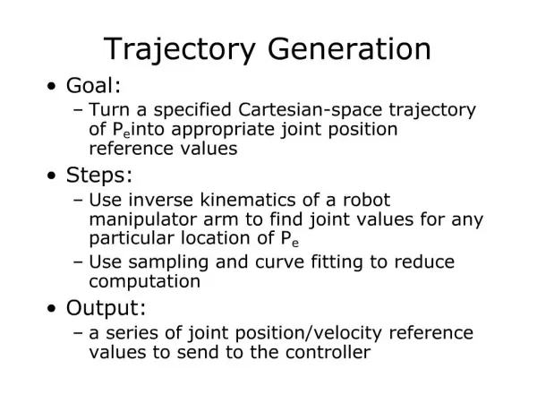
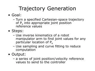
Introduction How to compute a trajectory in multidimensional space which describes the desired motion of a manipulator? How to move a manipulator from its initial position to some desired goal position in a smooth manner?
Trajectory • A time history of position, velocity, and acceleration for each DOF. • The system (not the user) will decide the exact shape of the path to get to the goal, the duration, the velocity profile, and other details. • A sequence of desired via points (frames which specify position and orientation of tool) can be given. • Path points include all the via points plus the initial and final points.
General Considerations • Each path point is specified in terms of a desired position and orientation of {T} relative to {S}. • Each of these points is converted into a set of desired joint angles. (Inverse kinematics). • A smooth function is found for each of the n joints which pass through the via points and end at the goal point. • The time required for each segment is the same for each joint.
Why Smooth Motion? • Increased wear on the mechanism • Vibrations A smooth function is continuous and has a continuous first (and second) derivatives.
Joint Space Scheme The path is specified in the joint space. • Easy to compute. • No problems with singularities. • Each path point is usually specified in terms of desired position and orientation of tool frame {T}. • Each of these via points is converted into a set of desired joint angles by inverse kinematics. Then a smooth function is fond so that all joints will reach the via point at the same time.
Several Possible Path Shapes for a Single Joint Goal position Initial position
Cubic Polynomials 4 constraints on : initial and final values : the function is continuous in velocity These 4 constraints can be satisfied by a polynomial of at least third degree.
Cubic Polynomials : combining with constraints The cubic polynomial that connects any initial joint angle position with any desired final position when the joint starts and finishes at zero velocity.
Example 7.1 A single-link robot with a rotary joint: Move the joint in a smooth manner from q=15 to q=75 in 3 seconds
Cubic Polynomials for a Path With Via Points • Each via point is specified in terms of a desired position and orientation of {T} relative to {S}. • Each of these via points is converted into a set of desired joint angles. (Inv. Kinematics). • Consider the problem of computing cubics which connect the via point values for each joint together in a smooth way.
Cubic Polynomials for a Path With Via Points : some known velocity at the via points : the four equations describing general cubic
Cubic Polynomials for a Path With Via Points Solving for ai we obtain Connects any initial and final positions with any initial and final velocities
How to Specify Desired Velocity at the Via Points? Several ways: • The user specifies the desired velocity at each via point in terms of a Cartesian linear and angular velocity of {T} at that instant. • The system automatically chooses the velocities at the via points. • The system automatically chooses the velocities at the via points in such a way as to cause the acceleration at the via points to be continuous.
A simple heuristic Tangents to the curve at each via points If the slope of these lines changes sign at the via point, choose zero velocity, if the slope of these lines does not change sign, choose the average of the two slopes as the via velocity.
Higher Order Polynomials • If we wish to be able to specify the position, velocity, and acceleration at the beginning and end of a path segment, a quintic polynomial is required.
Higher Order Polynomials :the constraints are given as
Higher Order Polynomials The solution for a linear set of equations with six unknowns:
Linear Interpolation Another choice of path is linear: Discontinuous velocity increase at the beginning and discontinuous velocity decrease at the end of the motion, requiringinfinite acceleration.
Linear Function With Parabolic Blends Constant acceleration The linear function and the two parabolic functions are splined together so that the entire path is continuous in position and velocity.
Linear Function With Parabolic Blends The parabolic blends have the same duration, are symmetric about the halfway point in time, and the halfway point in position.
Linear Function With Parabolic Blends The velocity at the end of the blend region must equal the velocity of the linear section. :One choice is. : the constraints on acceleration When equality occurs, the linear portion has shrunk to zero length.
Example 7.3 Two possible choice of linear path with parabolic blends for the path described in example 7.1
Linear Function With Parabolic Blends for a Path With Via Points Linear function connects the via points and parabolic blend regions are around each via point
Linear Function With Parabolic Blends for a Path With Via Points For 3 neighboring path points: j,k,l : duration of blend region at K : duration of linear region between j,k : overall duration of segment connecting j,k : velocity during linear portion : acceleration during the blend
Linear Function With Parabolic Blends for a Path With Via Points We can compute the blend time:
Linear Function With Parabolic Blends for a Path With Via Points The first and the last segments might be handled slightly different since an entire blend region must be counted in the segment’s time duration: This can be solved for blend time at initial point as:
The Path Generator • The results of computations constitute a plan for the trajectory. At execution time the path generator will use these numbers to compute , ,
Use of Pseudo Via Points to Create a Through Point Via points are not actually reached unless manipulator comes to stop. If we wish exactly passing through a point without stopping, the system may replace via point with 2 pseudo via points. A path point through which we force the manipulator to pass exactly!
Cartesian Space Schemes • We can specify the spatial shape of the path between path points. (Straight, circular, sinusoidal, …). • Each path point is specified in terms of position and orientation of tool frame relative to station frame. • This scheme is more computationally expensive because inverse kinematics must be solved at the path update rate.
Cartesian Straight Line Motion A spatial path which causes the tip of the tool to move through space in a straight line can be defined By: • Choosing many via points close together on a line. or • Using Cartesian motion functions to specify a path.
Cartesian Straight Line Motion • We may use a spline of linear function with parabolic blends for Cartesian motion. However as a rotation matrix must be composed of orthonormal columns and this condition would not be guaranteed if constructed by linear interpolation.
Angle-axis Representation Angle-axis representation can be used to specify an orientation with 3 numbers. ( for example Euler angles) If we combine this representation with Cartesian position we will have a 6x1 matrix: Now we can describe spline functions which smoothly move these 6 quantities from path point to path point as function of time
Angle-axis representation Note: Angle-axis representation is not unique Constraints: The blend time for each degree of freedom must be the same to ensure that the motion of all dof will be straight line in space. Hence we specify blend time and then compute the acceleration.
Geometric Problems With Cartesian Paths • Cartesian path are prone to various problems related to work space and singularities. • Intermediate points unreachable • High joint rate near singularity • Start and goal reachable in different solutions
Workspace violation Cartesian Path Problem Type I Intermediate points unreachable Moving from A to B would be no problem in joint space, but the straight path contains un-reachable points in Cartesian motion.
Near singular configuration Cartesian Path Problem Type II High joint rate near singularity
Joint limits Cartesian Path Problem Type III Start and goal reachable in different solutions
Next Course: Robot Programming Amirkabir University of TechnologyComputer Engineering & Information Technology Department