Solving Sudoku with Simulated Annealing
140 likes | 462 Vues
Solving Sudoku with Simulated Annealing. Bret Wilson. What is Simulated Annealing?. Analog of physical process of annealing in metals Heat, then cool slowly Start with random configuration Try nearby neighbors Lower temperature = become pickier. Heuristic.

Solving Sudoku with Simulated Annealing
E N D
Presentation Transcript
Solving Sudoku with Simulated Annealing Bret Wilson
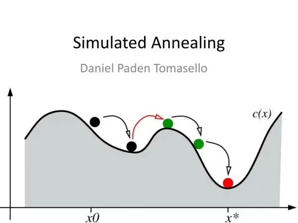
What is Simulated Annealing? • Analog of physical process of annealing in metals • Heat, then cool slowly • Start with random configuration • Try nearby neighbors • Lower temperature = become pickier
Heuristic • Only consider states in which each small square has exactly 1 of each digit 0 – 9 • Why? It’s trivial to solve either small squares, rows, or columns by themselves – I chose small squares. • -1 point for each different number in each row and column • Minimum (best) score = -9 x 9 x 2 = -162
Choosing a new state • Swap any 2 digits in same small square -> candidate • Accept new state if e-∆S/T – R > 0 • (Metropolis-Hastings Algorithm) • R is random number in range [0,1] • Always accept better states • Accept worse states more often when T is higher
Example • ∆S = -1 • e-∆S/T will always be > 1, no matter what T and R are. • So we accept.
Annealing Schedule • What should our initial value for T be? • Can find by trial and error • How fast should we decrease T? • Linear: T <= T – i where i > 0 • Geometric progression: T <= c*T where 0 < c < 1 • Change T based on current score
Pseudocode currState<= createInitialState() currScore <= score(currState) bestState<= currState bestScore <= currScore while (T > END) newState <= generateNeighbor(currState) newScore <= score(newState) if (exp((currScore - newScore)/T) - rand(0,1) > 0) currState <= newState currScore <= newScore if (currScore < bestScore) bestState <= currState bestScore <= currScore T <= c*T return bestState
Pros + Cons of Simulated Annealing • Good: Quickly finds a minimum • Bad: May not find global minimum (best solution) • Increasing temperature makes it slower, but less likely we will get stuck in local minimum
References • Carr, Roger. "Simulated Annealing." From MathWorld--A Wolfram Web Resource, created by Eric W. Weisstein. http://mathworld.wolfram.com/SimulatedAnnealing.html • “Simulated Annealing.” Wikipedia. http://en.wikipedia.org/wiki/Simulated_annealing • “Simulated Annealing Applet.” Heaton Research. http://www.heatonresearch.com/articles/64/page1.html
