Download
1 / 62
620 likes | 862 Vues
Chapter 14: Chi-Square Procedures. 14.1 – Test for Goodness of Fit. ( 2 ). Chi-square test for goodness of fit:. Used to determine if what outcome you expect to happen actually does happen. Count of actual results. Observed Counts:. Expected Counts:. Count of expected results.

E N D
(2) Chi-square test for goodness of fit: Used to determine if what outcome you expect to happen actually does happen Count of actual results Observed Counts: Expected Counts: Count of expected results To find the expected counts multiply the proportion you expect times the sample size
Note: Sometimes the probabilities will be expected to be the same and sometimes they will be expected to be different
Chi-square test for goodness of fit: Don’t need! P: H: Ho: All of the proportions are as expected HA: One or more of the proportions are different from expected A: all expected counts are ≥ 5 N: GOF test T: df = k – 1 categories
Properties of the Chi-distribution: • Always positive (being squared) • Skewed to the right • Distribution changes as degrees of freedom change
Properties of the Chi-distribution: • Always positive (being squared) • Skewed to the right • Distribution changes as degrees of freedom change • Area is shaded to the right
Calculator Tip! Goodness of Fit L1: Observed L2: Expected L3: (L1 – L2)2 / L2 List – Math – Sum – L3
P(2 > #) Calculator Tip! 2nd dist - 2cdf(2, big #, df)
Example #1 A study yields a chi-square statistic value of 20 (2 = 20). What is the P value of the test if the study was a goodness-of-fit test with 12 categories?
Example #1 A study yields a chi-square statistic value of 20 (2 = 20). What is the P value of the test if the study was a goodness-of-fit test with 12 categories? 0.025 < P < 0.05 Or by calc: 2nd dist - 2cdf(2, big #, df) 2cdf(20, 10000000, 11) = 0.04534
Example #2 A geneticist claims that four species of fruit flies should appear in the ratio 1:3:3:9. Suppose that a sample of 480 flies contains 25, 92, 68, and 295 flies of each species, respectively. Find the chi-square statistic and probability. 25 92 68 295 480/16 3 480/16 480/16 3 480/16 9 30 90 90 270 0.833 0.044 5.378 2.315 0.833 + 0.044 + 5.378 + 2.315 = 8.57
P(2 > 8.57) = df = 4 – 1 = 3
P(2 > 8.57) = df = 4 – 1 = 3 .025 < P(2 > 8.57) < 0.05 Or by calc: 2cdf(8.57, 10000000, 3) = 0.03559
Example #3 The number of defects from a manufacturing process by day of the week are as follows: The manufacturer is concerned that the number of defects is greater on Monday and Friday. Test, at the 0.05 level of significance, the claim that the proportion of defects is the same each day of the week. The proportion of defects from a manufacturing process is the same Mon-Fri H: Ho: HA: The proportion of defects from a manufacturing process is not the same Mon-Fri (on one day or more)
A: Expected Counts
A: Expected Counts 30 30 30 30 30 Expected 150 errors total. 150 5 = 30 N: Chi-Square Goodness of Fit
T: 30 30 30 30 30 Expected (O – E)2 E 2 = = 7.533
O: P(2 > 7.533) = df = 5 – 1 = 4
O: P(2 > 7.533) = df = 5 – 1 = 4 0.10 < P(2 > 7.533) > 0.15 Or by calc: 2cdf(7.533, 10000000, 4) = 0.1102
M: P ___________ > 0.1102 0.05 Accept the Null
S: There is not enough evidence to claim the proportion of defects from a manufacturing process is not the same Mon-Fri (on one day or more)
To compare two proportions, we use a 2-Proportion Z Test. If we want to compare three or more proportions, we need a new procedure.
Two – Way Table: • Organize the data for several proportions • R rows and C columns • Dimensions are r x c
To calculate the expected counts, multiply the row total by the column total, and divide by the table total: Row total x Column total table total Expected count = (r – 1)(c – 1) Degrees of Freedom:
Chi-Square test for Homogeneity: Compare two or more populations on one categorical variable Ho: The proportions are the same among all populations Ha: The proportions are different among all populations Conditions: SRS Expected Counts are ≥ 5
Chi-Square test for Association/Independence: Two categorical variables collected from a single population Ho: There is no association between two categorical variables (independent) Ha: There is an association (dependent) Conditions: SRS Expected Counts are ≥ 5
Calculator Tip! Test for Homogeneity/Independence 2nd – matrx – edit – [A] – rxc – Table info Then: Stat – tests –2–test Observed: [A] Expected: [B] Calculate Note: Expected: [B] is done automatically!
Example #1 The table shows the number of people in each grade of high school who preferred a different color of socks. 18 18 20 15 15 12 14 56 a. What is the expected value for the number of 12th graders who prefer red socks? 20 x 14 56 Row total x Column total table total = 5 Expected count = =
Example #1 The table shows the number of people in each grade of high school who preferred a different color of socks. b. Find the degrees of freedom. (r – 1)(c – 1) (3 – 1)(4 – 1) (2)(3) 6
Example #2 An SRS of a group of teens enrolled in alternative schooling programs was asked if they smoked or not. The information is classified by gender in the table. Find the expected counts for each cell, and then find the chi-square statistic, degrees of freedom, and its corresponding probability. 70 147 79 138 217 Expected Counts: Row total x Column total table total 70 x 79 217 70 x 138 217 = 25.484 44.516 = 147 x 79 217 147 x 138 217 53.516 93.484 = =
Expected Counts: 25.484 44.516 53.516 93.484 (O – E)2 E 2 = = 0.56197 (23 – 25.484)2 25.48 (47 – 44.516)2 44.516 (56 – 53.516)2 53.516 (91 – 93.484)2 93.484 + + +
Expected Counts: 25.484 44.516 53.516 93.484 (O – E)2 E 2 = = 0.56197 Degrees of Freedom: (r – 1)(c – 1) = (2 – 1)(2 – 1) = (1)(1) = 1 P(2 > 0.56197) =
Expected Counts: 25.484 44.516 53.516 93.484 (O – E)2 E 2 = = 0.56197 Degrees of Freedom: (r – 1)(c – 1) = (2 – 1)(2 – 1) = (1)(1) = 1 P(2 > 0.56197) = More than 0.25 OR: 0.4535
Example #3 At a school a random sample of 20 male and 16 females were asked to classify which political party they identified with. Are the proportions of Democrats, Republicans, and Independents the same within both populations? Conduct a test of significance at the α = 0.05 level. H: Ho: The proportions are the same among males and females and their political party HA: The proportions are different among males and females and their political party
A: SRS (says) Row total x Column total table total Expected Counts 5 20 16 36 15 3 18 20 x 18 36 20 x 15 36 20 x 3 36 = 10 8.33 1.67 = = 16 x 18 36 16 x 15 36 16 x 3 36 8 6.67 1.33 = = = Not all are expected counts are 5, proceed with caution!
N: Chi-Square test for Homogeneity
T: Expected (O – E)2 E 2 = = 0.855 (11 – 10)2 10 (7 – 8)2 8 (7 – 8.33)2 8.33 (8 – 6.67)2 6.67 (2 – 1.67)2 1.67 (1 – 1.33)2 1.33 + + + + +
O: P(2 > 0.855) = Degrees of Freedom: (r – 1)(c – 1) = (2 – 1)(3 – 1) = (1)(2) = 2
O: P(2 > 0.855) = More than 0.25 Degrees of Freedom: (r – 1)(c – 1) = (2 – 1)(3 – 1) = (1)(2) = 2 OR: P(2 > 0.855) = 0.6521
M: P ___________ > 0.05 0.6521 Accept the Null