Download

1 / 42
420 likes | 452 Vues
Learn about chi-square procedures for categorical variables, including tests for goodness of fit, homogeneity of populations, and association/independence. Understand how to analyze sample distributions against hypothesized population distributions.

E N D
CHAPTER 14Inference for Distributions of Categorical Variables:Chi-square Procedures
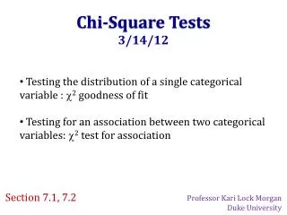
3 Unique Chi-Square Tests • Chi-square test for goodness of fit • Allows us to determine whether a specified population distribution is valid • Different from other two in the calculator • Chi-square test for homogeneity of populations • (also called test for homogeneity of proportions) • Allows us to compare two or more population proportions • Chi-square test of association/independence • Allows us to determine whether the distribution of one variable has been influenced by another variable
SECTION 14.1Test for Goodness of Fit Could the observed counts for a categorical variable come from a certain hypothesized distribution?
Something to Start our Thoughts • Assume you roll a die 86 times and get 9 ones, 15 twos, 10 threes, 14 fours, 17 fives, and 21 sixes. • Is there any reason to question the fairness of this die? • What should the distribution look like? • Essentially, we have a hypothesized population distribution and we are trying to see whether this sample gives us any reason to doubt that the population distribution holds for this die.
chi-square (X2) test for goodness of fit • We use this to see if an observed sample distribution is significantly different in some way from the hypothesized population distribution. • Essentially, we are trying to see how “good” our sample data “fits” the suggested population distribution.
Chi-Squared Statistic • The chi-square (X2) statistic is calculated as follows: • X2 = sum[(observed - expected)2/expected]
Basic Properties of X2 • X2are only positive values. • The X2 distribution is not symmetrical. It is skewed to the right. • All X2tests are 1-tail tests. • In a goodness of fit test, the degrees of freedom are number of categories - 1.(n-1)
Like the t-distributions, there is a different X2 distribution for each degree of freedom.
Key Notes • The expected count is always obtained by multiplying the percent of the distribution times the sample size. • P-value is the area under the density curve to the right of X2 and large values of X2 are evidence against H0. • H0: Actual population percents (or proportions) are equal to the hypothesized percentages (props). In some cases, you may end up writing this out as a list. There is often no easy way to express the null hypothesis for the goodness of fit test. • Ha: The actual percentages (or proportions) are different from the hypothesized percentages (props). • Test of goodness of fit can only be used when • We have an SRS from the population of interest • all EXPECTED counts are at least 1 and at least 80% are greater than 5 (also expressed as no more than 20% of expected values are less than 5).
Using the Calculator • If you want to use the calculator, you need to enter your information into lists. • For sake of simplicity, enter your observed values into L1 and your expected values into L2. • To find your X2 statistic you must: • Find Sum. Which is under 2nd list > math > 5. Then do sum((L1 - L2)2/ L2) and this gives you your Chi-squared statistic. • If you would like to see a list of your observed - expected values, for L3, enter L1 - L2 and just store them in L3 and you can use L3 instead of (L1 - L2)
More Calculator • For finding the P-value, go to 2nd Vars X2cdf and plug in the X2 statistic which is the sum of the components of X2, then the ending value, and last the degrees of freedom • X2cdf(x2, E99, df) calculator gives you your P-value • As long as your calculator isn’t too old, you also have the option of using X2 GOF-Test
Conclusions • As always, low P-values lead us to reject the null hypothesis. We will use the same standards as before when making our decisions. • Don’t forget to make a contextual conclusion in the context of the problem.
Follow Up Analysis • When you are making your conclusions, if you reject the null hypothesis, make sure you look at the individual components of chi-square to see which categories caused chi-square to be large enough to reject the null hypothesis and comment on these categories and their large difference between what was expected and what actually occurred.
An Informal EXAMPLE(meaning not all steps are covered) • In statistics, there are usually 15% A’s, 50% B’s, 20% C’s, 10% D’s, and 5% F’s for each test. • On the most recent test, there were 15 A’s, 8 B’s, 5 C’s, 5 D’s, and 9 F’s. • Is there sufficient evidence to suggest that the results of this test were significantly different than the standard grades?
Wrapping up the Example • sum(L4)=44.2619 • P-value =X2cdf(44.2619, E99, 4)=5.6603E-9 = 0.0000000056603 • This indicates that these test results are far from what we would expect. However, we had 40% of our expected values below 5 so these results should be interpreted with caution.
Example: The Graying of America • In recent years, the expression “the graying of America” has been used to refer to the belief that with better medicine and healthier lifestyles, people are living longer, and consequently a larger percentage of the population is of retirement age. We want to investigate whether this perception is accurate. The distribution of the U.S. population in 1980 is shown in the table on the next slide. We want to determine if the distribution of age groups in the United States in 1996 has changed significantly from the 1980 distribution.
Step 1: Parameters • Before we even see data from our sample (in 1996) we can establish our hypotheses based on the scenario described • H0: the age group distribution in 1996 is the same as the 1980 distribution • Ha: the age group distribution in 1996 is different from the 1980 distribution • The idea of this test (goodness of fit) is this: we compare the observed counts for a sample from the 1996 population with the counts that would be expected if the 1996 distribution were the same as the 1980 distribution, that is, if H0 were in fact true. The 1980 distribution is the population. The more the observed counts differ from the expected counts, the more evidence we have to reject H0 and conclude that the population distribution in 1996 is significantly different from that of 1980.
A random sample of 500 U.S. residents in 1996 is selected and the age of each subject is recorded. The counts and percents in each age group category are shown in the following table
Step 2: Conditions • SRS—We know that we have a random sample of 500 individuals from 1996. These should be representative of all U.S. resident in 1996 provided an SRS was used. • We also want to make sure that all EXPECTED counts are sufficiently large. As seen below, they are plenty big enough.
Step 3: Calculations • With a goodness of fit test, it is always a good idea to graph the data before proceeding with the test. To do this, create a segmented or side-by-side bar graph to show the comparison effectively. • In order to determine whether the distribution has changed since 1980, we need a way to measure how well the observed counts (O) from 1996 fit the expected counts (E) under H0. The procedure is to calculate (O-E)2/E for each age category and then add up these terms to arrive at our chi-square (X2) statistic. The larger the differences between the observed and expected values, the larger X2 will be, and the more evidence there will be against H0.
Step 3 (continued): Calculations Since there are 4 age groups, we have 4-1 or 3 degrees of freedom. We use df=3 and X2=8.2275 to determine that our P-value is 0.0415
Step 4: Interpretation • Based on our low P-value, we will reject the null hypothesis. • The probability of observing a result as extreme as the one we actually observed, by chance alone, is less than 5%. • We conclude that the population distribution in 1996 is significantly different from the 1980 distribution. • As a follow up analysis, we note that the 0 to 24 age group is considerably smaller than we would expect (if nothing had changed since 1980) in a group of 500 people. This age group was the most noticeably different in 1996 as compared to 1980.
SECTION 14.2Inference for Two-Way Tables • Chi-square test for homogeneity of populations • Does a single categorical variable have the same distribution in two or more distinct populations? • Chi-square test of association/independence • Are two categorical variables associated or independent?
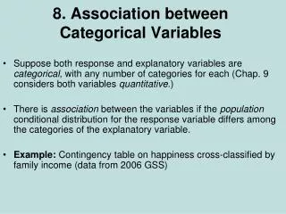
The Big Ideas • The relationship between two categorical variables measured on the same individuals is displayed in a two-way table of counts. • The chi-square test assesses whether the relationship between two categorical variables is statistically significant. The test is based on comparing observed counts in the two-way table to the counts we would expect if knowing the value of one variable gives no information about the other. • Large values of the chi-square statistic are evidence against the null hypothesis of no relationship. That is, the test is always one-sided. P-values come from the chi-square distributions. • Because the chi-square test does not look for any particular form of relationship, be sure to describe the observed relationship along with the test.
Chi-square test for Two-way tables A table is used and laid out by Rows vs Columns. For example a 3x2 table has 3 rows and 2 columns. Rows being horizontal and columns being vertical. Generically, our hypotheses will be: Ho: there is no relationship between 2 categorical variables Ha: that there is a relationship between 2 categorical variables Expected count = row total x column total table total If the observed counts are far from the expected counts, that is evidence against Ho. You can safely use the chi-square test when the at least 80% of expected counts are greater than 5 and all expected counts are 1 or greater. Of course you also need to make sure the data comes from one or more SRSs (depending on the scenario).
Calculator for Two-Way Tables • Go to matrix and plug the observed values into matrix A (row is first number column is second) • Ex. r=3 c=2; 3x2 matrix • Then go to Stat:Tests X2 test • Observed: [A] and it plugs the expected values into matrix [B] after hitting calculate • It gives you your X2, your P-value and your degrees of freedom which are (r-1)(c-1).
Let’s try one INFORMAL example (like before, that means this won’t include all steps):Is there a relationship between your class and your preference for lunch? WHICH TEST DO WE USE? Chi-square test of association/independence
Observed vs. Expected The expected count for freshmen that bring their lunch 1113 x 690 / 2553 = 300.81 (Note: these are stored in Matrix [B] )
Running the Test Null hypothesis is that there is no relationship between high school class and lunch preference. The alternative is that there is a relationship between high school class and lunch preference. All individual expected counts are at least one (the lowest is 59.89) and since they are all at least 5 then we know that no more than 20% are less than 5. X2 = 269.33 P-value = 8.19 x 10-53 df = (r - 1)(c - 1) = (4-1)(4-1) = 9 Based on the extremely low P-value we reject the null hypothesis and are comfortable accepting the alternative hypothesis. This means that there is a relationship between a students grade level and their lunch preference.
DON’T FORGET:Follow Up Analysis You should do some follow up analysis of the differences between observed and expected values. This can be more challenging than in the previous section simply because you don’t get a chance to look at the components of chi-square unless you determine them individually. Instead, you can simply look at the most noticeable raw differences, calculate the component of chi-square for that cell, and see how big a part of your chi-square statistic this would be. This gives a better idea of how important that cell is to making the relationship significant. Essentially, if you reject the null hypothesis, make some comments about what aspects of the relationship led to a high enough chi-square value for this decision. In this case, the large difference in two cells (freshmen and seniors who go out to eat) were the main reason for a large chi-square statistic (127.58 and 62.78 respectively).
A Full Example: Health care: Canada and the United States • Canada has universal health care. The U.S. does not, but often offers more elaborate treatment to patients with access. How do the two systems compare in treating heart attacks? A comparison of random samples of 2600 U.S. and 400 Canadian heart attack patients found: “The Canadian patients typically stayed in the hospital one day longer (P-value<0.001), coronary angioplasty (11% vs. 29%, P-value<0.001), and coronary bypass surgery (3% vs. 14%, P-value<0.001).” • The study then looked at many outcomes a year after the heart attack. There was no significant difference in the patients’ survival rate. Another key outcome was the patients’ own assessment of their quality of life relative to what it had been before the heart attack. Here are the data for the patients who survived a year:
The two-way table shows the relationship between two categorical variables. The explanatory variable is the patient’s country and the response variable is the quality of life a year after a heart attack. The two-way table gives the counts for all 10 combinations of values of these variables. Each of the 10 counts occupies a cell of the table. It is hard to compare the counts because the U.S. sample is much larger. Here are the percents of each sample with each outcome: NOTICE ANYTHING STRIKINGLY DIFFERENT ABOUT THESE PERCENTS?
Be Careful With Analysis • Clearly, the first two categories don’t show any difference worth discussing. The last three categories are off by enough that we may be inclined to use procedures from previous chapters to “test” whether one particular category has a significant difference in proportions between the U.S. and Canada. If we did this, for example, with the “much worse” category, we would find that the proportions are significantly different (P-value=0.0047). • But is it surprising that one of five categories would differ by this much? • Really, it is “cheating” to pick out the largest of five differences and then test its significance as if it were the only comparison we had in mind.
So which test should we perform? • The chi-square test for homogeneity of populations. WHY? • Because our data comes from two distinct populations and we want to determine if there is a significant difference in quality of life after a heart attack in the two countries. • STEP 1: Parameters • The null hypothesis is that there is no difference between the distributions of outcomes in Canada and the United States. • H0: there is no relationship between nationality and quality of life • The alternative hypothesis is that there is a relationship but does not specify any particular kind of relationship. • Ha: there is some relationship between nationality and quality of life
Step 2: Conditions • SRS: The data came from independent random samples from the two populations of interest—Canadian and U.S. heart attach patients. • Expected counts are all well over 5 so there are no concerns. Show the expected counts.
Steps 3 & 4: Calculations and Interpretation • X2=11.725 • P-value = 0.0195 • df = (5-1)(2-1) = 4 • Since the P-value is so small, we will reject the null hypothesis. There is quite good evidence that the distributions of outcomes are different in Canada and the United States. • Follow-up analysis: The biggest contributor to our high chi-square statistic is for Canadians who report a much worse quality of life. That cell has a chi-square component of 6.766 which is over half of the total chi-square statistic. A higher proportion of Canadians report a much worse quality of life and this is the most important difference between the two countries.
One more quick example • The type of medical care that a patient receives sometimes varies with the age of the patient. For example, women should receive a mammogram and biopsy of any suspicious lump in the breast. Here are data from a study that asked whether women did receive these diagnostic tests when a lump in the breast was discovered. Which test should be done for this two-way table? Since a single sample was classified two ways (by age and whether or not a test was done) this setting requires a chi-square test for association/independence.
Running our Chosen TestSteps 1 & 2: Parameters & Conditions • Our null hypothesis is that there is no relationship between a women’s age and whether or not she has diagnostic testing done when a lump appears on her breast. • Our alternative is that there is a relationship between these two categorical variables. • Assuming that this study used an SRS when collecting the data, we should be fine using this test because all of the expected values are well over 5.
Steps 3 & 4: Calculations and Interpretation • X2=7.3668 • P-value = 0.0251 • df = (3-1)(2-1) = 2 • Based on the low P-value, we will reject the null hypothesis. • There is good evidence that the proportion of women in the population for whom the tests were done differs among the three age groups. • Comparing the expected values (to the right) to the observed values, we can see that the most notable difference is for the older group that did not get the test done. We can speculate as to why, but this test does not provide that type of information.