Steady-State Methods
Steady-State Methods. UCB EE219A Oct 29 2002 Joel Phillips, Cadence Berkeley Labs. Some artwork thanks to: K. Kundert. Steady-State Methods: Goals. Understand alternative way of analyzing differential equations Faster Application-Specific “Tie together” several numerical themes

Steady-State Methods
E N D
Presentation Transcript
Steady-State Methods UCB EE219A Oct 29 2002 Joel Phillips, Cadence Berkeley Labs Some artwork thanks to: K. Kundert
Steady-State Methods: Goals • Understand alternative way of analyzing differential equations • Faster • Application-Specific • “Tie together” several numerical themes • Circuit theory • Solution of ODEs/DAEs • Newton methods • Iterative solvers & preconditioning
Review: Solution of ODEs/DAEs • Given an ODE/DAE • Start with an initial condition • Pick a next time point (discretize time) • Compute next solution (Newton etc.) • Go to 3. and repeat till done
Good Questions For Transient Analysis • How does the circuit behave • When driven by a sinusoids (for a short time?) • When driven by a step input? • When driven by unstructured (i.e. a-periodic) inputs • Other time-domain characteristics • Delay, Risetime, Overshoot
Hard Questions for Transient Analysis • How does the circuit behave • When driven by sinusoid(s) for a very long time? (steady-state) • How much noise does the circuit introduce to a signal? • Where does the noise come from? Where does it go? • Other frequency-domain questions • Small-signal stability, Bode plot, pole-zero
Example Frequency-Domain Analysis TBR Model Not Positive Real
Why steady-state methods? • Speed • E.g., AC • Accuracy • E.g., distortion • Insight • E.g., stability • No choice! • RF noise
Prototypical steady-state analysis: AC • Linear Circuits • Apply a sinusoidal source at single frequency • Sweep the frequency of source (Bode/Nyquist plot) Small-signalsource Measuredresponse
AC via TRAN • Apply source • Solve IVP (Trap, Euler, etc.) • Wait till steady state is reached • Fourier-transform the output
Problem #1: Speed • Consider a 1Hz sinusoid applied to a resonant RLC circuit Transients must die out to avoidcorrupting steady-state Each period requires20-50 timepoints? Must simulate forminimum one secondpast transients
Problem #2: Accuracy • Widely used BAD method for Fourier analysis • Interpolate onto uniform timepoints, apply FFT • Problems • Detecting “onset” of steady-state • Polynomial interpolation creates high noise floors in Fourier analysis • Truncation errors corrupt spectrum • Aperiodicity/endpoint errors
How bad can it be? • Experiment: • Sample sinusoid at 256 random points • Interpolate onto uniform 1024-point grid • FFT • Looks good so far!!!
AC Linear Analysis Sinusoidalinput u • Consider linear problem • Recall: In the frequency-domain • Nice feature: work for all linear elements (e.g., transmission lines) Laplacetransform Fouriertransform Sinusoidal steady-state Fundamental AC analysis equation
AC Small-Signal for Nonlinear Circuits • Step 1: Find the DC operating point • In a circuit, this means find a set of currents, voltages that satisfy Kirchoff’s voltage & current laws, with all capacitors deleted and all inductors shorted (Recall that: DC operating point itself is very useful in circuit design…..)
AC Small-Signal for Nonlinear Circuits • Step 2: Linearize around the DC operating point • Assume the inputs are small perturbations around the DC point • Assume circuit response is in turn a small perturbation around the DC point (use Taylor series)
AC Small-Signal for Nonlinear Circuits • Step 3: Solve the AC analysis equation • Note: Fourier portion of analysis is exact • No truncation error • No aliasing errors • No periodicity errors
More Linear Analyses: Pole-Zero • Is the design stable? Poles all in left half-plane? Recall AC analysis: • Poles occur at (complex) such that • Solve eigenvalue problem by • Direct methods: QZ; or Krylov methods: Lanczos, Arnoldi (similar to GMRES!)
Thermal NoiseSource Noise appearsat output Noise Analysis • Lossy devices in circuit generate noise • Noise is: Stochastic (random) unwanted signal • Typical model: • Stationary Gaussian process characterized by power spectrum
White Noise Fourier Transform R(t,t) S(f ) Autocorrelation Spectrum f t • Noise at each time point is independent • Noise is uncorrelated in time • Spectrum is white • Examples: thermal noise, shot noise
Colored Noise Noise is correlated in time because of time constant Spectrum is shaped by frequency response of circuit Noise at different frequencies is independent (uncorrelated) Fourier Transform R(t,t) S(f ) Autocorrelation Spectrum f t Time correlationÛFrequency shaping
Possibly correlated “white” Gaussian processes Noise Analysis • Typical model • Assume “small” small signal analysis • Stationary Gaussian process characterized by power spectrum • Small-signal analysis with noise sources • Frequency-domain method: • Compute transfer function from each noise source to the observation point (output) [Same transfer functions as computed by AC] • Sum noise power contributions. Correlations will be correctly tracked.
AC-like Transfer Function Computation Output LinearizedCircuit Source 1 • Each source requires a transfer function analysis • Number of sources M number of devices • Too many solves! etc. Source M
Adjoint Analysis • Standard AC analysis to compute • Solve (expensive) • For any output desired, compute (cheap) • Key observation: • Adjoint analysis • One c, lots of b (or many more b than c) • Solve • For all the inputs (sources), compute
Output 1 Output 2 Output 3 Output 4 Forward Analysis: Circuit Interpretation For one input configuration, compute TF from to all possible outputs Input 1 LinearizedCircuit Input 2 Input 3
Output 1 Output 2 Output 3 Output 4 Adjoint Analysis: Circuit Interpretation For one output configuration, compute TF from all possible inputs Input 1 LinearizedCircuit Input 2 Input 3
Generalizations of Steady-State Analyses • Mostly ways of dealing with LARGE signal effects • i.e., NONLINEAR analysis • Examples: • Distortion • Frequency Conversion
+ - Distortion • Consider amplifier with cubic nonlinearity • Harmonic distortion • Intermodulation distortion
w w 1 2 Distortion Real life is more complicated with nonlinearfrequency-dependent terms, higher-order nonlinearities, and more complex inputs.
Frequency-Translation • Linear Mixer • Common confusion: frequency translation itself is a linear process (not nonlinear) • But all actual frequency-translating devices are nonlinear
Simple Nonlinear Steady-State Problems * • Compute harmonic distortion in the amplifier • Compute conversion gain in the mixer • Compute noise in either • All three are periodic-steady-state problems • (or periodic steady-state + small-signal analysis) *[intermodulation distortion is a quasi-periodic steady-state problem]
Periodic Steady-State • Assume general excitation by periodic inputs • In many cases, we expect a periodic solution [if we wait long enough…] • Recall: periodic functions have a Fourier-series representation (sum of sine and cosines) • Why not solve for the periodic solution directly?
Periodic Steady-State Computation • Apply a sinusoid or other periodic input signal • Find the periodic response • Time-domain solution over one “fundamental” period • Or spectrum: Fourier coefficients at fundamental + harmonics • Sound familiar???? • Recall: in AC, we solved directly for the Fourier response (“fundamental”). No higher harmonics arise because system was linear. • Need: • Steady-state “equations” ala • FAST & ACCURATE way of solving equations
IVP vs BVP • No problem specified with differential equations is complete without boundary condition • Before: Solving an Initial Value Problem (IVP) • What about: • Example of a boundary-value problem (BVP)
Note on PBCs • If solution to DAE is unique, then solution on one period determines solution for all time • Both the shooting method and spectral interval methods (harmonic balance) use this fact • From knowledge of solution at one timepoint, can easily construction solution over entire period by solving IVP • We will exploit this in the shooting method
Enforcing PBCs • Approach 1: Build BCs in basis function • Example: Fourier series satisfy periodic boundary conditions • Approach 2: Write extra equations • PBC
PSS Algorithm #1: Harmonic Balance • Periodic solution can be expressed in terms of Fourier series with fundamental frequency • Pick -- OR -- (real solutions please!)
PSS Algorithm #1: Harmonic Balance • Pick • Want to solve • Clever trick: spectral derivatives!
Spectral Differentiation • Recall • Works on any function • With suitable technical conditions • Spectral differentiation is exact for sinusoids!!!! Occasional linearity confusion:Linear circuit sinusoids do not interact.Differentiation acts on signals, not the nonlinear functions, so Fourier analysisworks fine.
How good is spectral differentiation? Plot vs. on finite difference grid
Aside on Weighted Residuals • Many numerical methods you know are weighted residual methods • General scheme to solve • Pick basis functions • Ansatz: • Select weighting functions • Force
Weighted Residuals: Examples • Least-Squares • GMRES • Collocation: • Original equations satisfied exactly at some “points” • BDF collocates derivatives • Galerkin: • Residual orthogonal to basis space (or some other space) • Krylov-based Model Reduction
Harmonic Balance: Equation Formation • Enforce • Galerkin (true spectral method) • Point collocation (“pseudo-spectral method”) • Force at selected timepoints • Which ones? Time for another trick…..
Differentiation and the DFT • Fourier transform (DFT) relates solution at discrete points to Fourier coefficients [strictly speaking, we are evaluating the Fourier integral via quadratureusing the trapezoidal rule. Useful fact: trapezoidal rule is the best rule (spectrally accurate!) for quadrature on a circle. ]
Differentiation and the FFT • Derivative in Fourier space: • DFT-based differentiation formula • We can evaluate a DFT fast using an FFT • Suggests selecting timepoints to be evenly spaced
Equation Structure • BVP becomes • Jacobian with (sorta looks like AC, doesn’t it???)
Equation Solution • We need to solve • These matrices are dense in either Fourier- or real- space LU factorization is bad news • They are potentially very large • Yet a matrix-vector product can be done fast • Ideal candidate for iterative solution methods (GMRES!) • Good preconditioners are necessary, but hard to construct
Historical Note about Device Evaluation • Once upon a time…..microwave/RF simulators were purely frequency-domain…..like AC. • Problem: This required frequency-domain transistor models. • At some point it was noticed that the devices could be evaluated in the time-domain (with equations written in frequency domain) by using Fourier transforms.