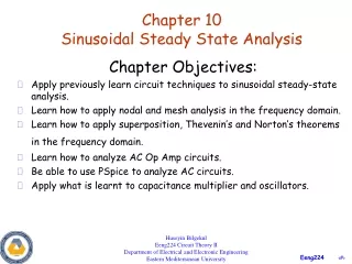
Sinusoidal Steady-state Analysis

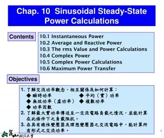
1. Sinusoidal Steady-state Analysis • Complex number reviews • Phasors and ordinary differential equations • Complete response and sinusoidal steady-state response • Concepts of impedance and admittance • Sinusoidal steady-state analysis of simple circuits • Resonance circuit • Power in sinusoidal steady –state • Impedance and frequency normalization

2. Complex number reviews Complex number Magnitude Phase or angle In polar form or The complex number can be of voltage, current, power, impedance etc.. in any circuit with sinusoid excitation. Operations: Add, subtract, multiply, divide, power, root, conjugate

3. Phasors and ordinary differential equations A sinusoid of angular frequency is in the form Theorem The algebraic sum of sinusoids of the same frequency and of their derivatives is also a sinusoid of the same frequency Example 1

4. Phasors and ordinary differential equations phasor Example 2 phasor form

5. Phasors and ordinary differential equations Ordinary linear differential equation with sinusoid excitation Lemma: Re[.. ] is additive and homogenous

6. Phasors and ordinary differential equations Application of the phasor to differential equation Let substitute in (1) yields

7. Phasors and ordinary differential equations even power odd power

8. Phasors and ordinary differential equations Example 3 From the circuit in fig1 let the input be a sinusoidal voltage source and the output is the voltage across the capacitor. Fig1

9. Phasors and ordinary differential equations KVL Particular solution

10. Phasors and ordinary differential equations

11. Complete response and sinusoidal steady-state response Complete reponse = sinusoid of the same input frequency (forced component) =solution of homogeneous equation (natural component) (for distinct frequencies)

12. Complete response and sinusoidal steady-state response Example 4 For the circuit of fig 1, the sinusoid input is applied to the circuit at time . Determine the complete response of the Capacitor voltage. C=1Farad, L=1/2 Henry, R=3/2 ohms. From example 3 Initial conditions

13. Complete response and sinusoidal steady-state response Characteristic equation Natural component Forced component From (2)

14. Complete response and sinusoidal steady-state response The complete solution is

15. Complete response and sinusoidal steady-state response The complete solution is

16. Complete response and sinusoidal steady-state response Sinusoidal steady-state response In a linear time invariant circuit driven by a sinusoid source, the response Is of the form Irrespective of initial conditions ,if the natural frequencies lie in the left-half complex plane, the natural components converge to zero as and the response becomes close to a sinusoid. The sinusoid steady state response can be calculated by the phasor method.

17. Complete response and sinusoidal steady-state response Example 5 Let the characteristic polynomial of a differential a differential equation Be of the form The characteristic roots are and the solution is of the form In term of cosine The solution becomes unstable as

18. Complete response and sinusoidal steady-state response Example 6 Let the characteristic polynomial of a differential a differential equation Be of the form The characteristic roots are and the solution is of the form and The solution is oscillatory at different frequencies. If the output is unstable as

19. Complete response and sinusoidal steady-state response Superposition in the steady state If a linear time-invariant circuit is driven by two or more sinusoidal sources the output response is the sum of the output from each source. Example 7 The circuit of fig1 is applied with two sinusoidal voltage sources and the output is the voltage across the capacitor.

20. Phasors and ordinary differential equations KVL Differential equation for each source

21. Phasors and ordinary differential equations The particular solution is where

22. Complete response and sinusoidal steady-state response Summary A linear time-invariant circuit whose natural frequencies are all within the open left-half of the complex frequency plane has a sinusoid steady state response when driven by a sinusoid input. If the circuit has Imaginary natural frequencies that are simple and if these are different from the angular frequency of the input sinusoid, the steady-state response also exists. The sinusoidal steady state response has the same frequency as the input and can be obtained most efficiently by the phasor method

23. Concepts of impedance and admittance Properties of impedances and admittances play important roles in circuit analyses with sinusoid excitation. Phasor relation for circuit elements Fig 2

24. Concepts of impedance and admittance Resistor The voltage and current phasors are in phase. Capacitor The current phasor leads the voltage phasor by 90 degrees.

25. Concepts of impedance and admittance Inductor The current phasor lags the voltage phasor by 90 degrees.

26. Concepts of impedance and admittance Definition of impedance and admittance The driving point impedance of the one port at the angular frequency is the ratio of the output voltage phasor V to the input current phasor I or The driving point admittance of the one port at the angular frequency is the ratio of the output current phasor I to the input voltage phasor V or

27. Concepts of impedance and admittance

28. Sinusoidal steady-state analysis of simple circuits In the sinusoid steady state Kirchhoff’s equations can be written directly in terms o voltage phasors and current phasors. For example: If each voltage is sinusoid of the same frequency

29. Sinusoidal steady-state analysis of simple circuits Series parallel connections In a series sinusoid circuit Fig 3

30. Sinusoidal steady-state analysis of simple circuits In a parallel sinusoid circuit Fig 4

31. Sinusoidal steady-state analysis of simple circuits Node and mesh analyses Node and mesh analysis can be used in a linear time-invariant circuit to determine the sinusoid steady state response. KCL, KVL and the concepts of impedance and admittance are also important for the analyses. Example 8 In figure 5 the input is a current source Determine the sinusoid steady-state voltage at node 3 Fig 5

32. Node and mesh analyses KCL at node 1 KCL at node 2 KCL at node 3

33. Node and mesh analyses Rearrange the equations By Crammer’s Rule

34. Node and mesh analyses Since Then and the sinusoid steady-state voltage at node 3 is Example 9 Solve example 8 using mesh analysis Fig 6

35. Node and mesh analyses KVL at mesh 1 KVL at mesh 2 KVL at mesh 3

36. Node and mesh analyses Rearrange the equations By Crammer’s Rule

37. Node and mesh analyses Since Then and the sinusoid steady-state voltage at node 3 is The solution is exactly the same as from the node analysis

38. Resonance circuit Resonance circuits form the basics in electronics and communications. It is useful for sinusoidal steady-state analysis in complex circuits. Impedance, Admittance, Phasors Figure 7 show a simple parallel resonant circuit driven by a sinusoid source. Fig 7

39. Resonance circuit The input admittance at the angular frequency is The real part of is constant but the imaginary part varies with frequency At the frequency the susceptance is zero. The frequency is called the resonant frequency.

40. Resonance circuit The admittance of the parallel circuit in Fig 7 is frequency dependant Fig 8 Susceptance plot

41. Resonance circuit Fig 9 Locus of Y Locus of Z

42. Resonance circuit The currents in each element are and If for example The admittance of the circuit is The impedance of the circuit is

43. Resonance circuit The voltage phasor is Thus Fig 10

44. Resonance circuit and Similarly if The voltage and current phasors are Note that it is a resonance and Fig 11

45. Resonance circuit The ratio of the current in the inductor or capacitor to the input current is the quality factor or Q-factor of the resonance circuit. Generally and the voltages or currents in a resonance circuit is very large! Analysis for a series R-L-C resonance is the very similar

46. Power in sinusoidal steady-state The instantaneous power enter a one port circuit is The energy delivered to the in the interval is Fig 12

47. Power in sinusoidal steady-state Instantaneous, Average and Complex power In sinusoidal steady-state the power at the port is where If the port current is where

48. Power in sinusoidal steady-state Then Fig 13

49. Power in sinusoidal steady-state • Remarks • The phase difference in power equation is the impedance angle • Pav is the average power over one period and is non negative. But p(t) may be negative at some t • The complex power in a two-port circuit is • Average power is additive

50. Power in sinusoidal steady-state • Maximum power transfer The condition for maximum transfer for sinusoid steady-state is that The load impedance must be conjugately matched to the source imedance • Q of a resonance circuit For a parallel resonance circuit (Valid for both series and parallel resonance circuits)