Ch4 Sinusoidal Steady State Analysis

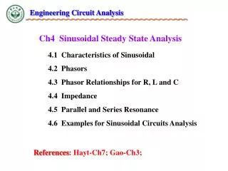
1. Engineering Circuit Analysis Ch4 Sinusoidal Steady State Analysis 4.1Characteristics of Sinusoidal 4.2 Phasors 4.3Phasor Relationships for R, L and C 4.4 Impedance 4.5 Parallel and Series Resonance 4.6 Examples for Sinusoidal Circuits Analysis References: Hayt-Ch7; Gao-Ch3;

2. Ch4 Sinusoidal Steady State Analysis • Any steady state voltage or current in a linear circuit with a sinusoidal source is a sinusoid • All steady state voltages and currents have the same frequency as the source • In order to find a steady state voltage or current, all we need to know is its magnitude and its phase relative to the source (we already know its frequency) • We do not have to find this differential equation from the circuit, nor do we have to solve it • Instead, we use the concepts of phasors and complex impedances • Phasors and complex impedances convert problems involving differential equations into circuit analysis problems  Focus on steady state; 􀂄 Focus on sinusoids.

3. Ch4 Sinusoidal Steady State Analysis 4.1Characteristics of Sinusoidal Key Words: Period: T , Frequency: f , Radian frequency  Phase angle Amplitude: Vm Im

4. v、i t t1 t2 0 Ch4 Sinusoidal Steady State Analysis 4.1Characteristics of Sinusoidal Both the polarity and magnitude of voltage are changing.

5. v、i Vm、Im t 0  2 Ch4 Sinusoidal Steady State Analysis 4.1Characteristics of Sinusoidal Radian frequency(Angular frequency):= 2f = 2/T (rad/s） Period: T — Time necessary to go through one cycle. (s) Frequency: f— Cycles per second. (Hz) f= 1/T Amplitude: Vm Im i = Imsint， v=Vmsint

6. Effective Value of a Periodic Waveform Ch4 Sinusoidal Steady State Analysis 4.1Characteristics of Sinusoidal Effective Roof Mean Square (RMS) Value of a Periodic Waveform — is equal to the value of the direct current which is flowing through an R-ohm resistor. It delivers the same average power to the resistor as the periodic current does.

7. Phase angle <0 0 Ch4 Sinusoidal Steady State Analysis 4.1Characteristics of Sinusoidal Phase (angle)

8. — v(t) leads i(t) by (1 - 2), or i(t) lags v(t) by (1 - 2) — v(t) lags i(t) by (2 - 1), or i(t) leads v(t) by (2 - 1) v、i v、i v、i Out of phase。 In phase. v v v i i i t t t Ch4 Sinusoidal Steady State Analysis 4.1Characteristics of Sinusoidal Phase difference

9. 360°—— does not change anything. 90° —— change between sin & cos. 180°—— change between + & - Ch4 Sinusoidal Steady State Analysis 4.1Characteristics of Sinusoidal Review The sinusoidal waves whose phases are compared must: ① Be written as sine waves or cosine waves. ② With positive amplitudes. ③ Have the same frequency.

10. Find Ch4 Sinusoidal Steady State Analysis 4.1Characteristics of Sinusoidal Phase difference P4.1, If

11. v、i v i • • • t  -/3 /3 Ch4 Sinusoidal Steady State Analysis 4.1Characteristics of Sinusoidal Phase difference P4.2,

12. Ch4 Sinusoidal Steady State Analysis 4.2Phasors A sinusoidal voltage/current at a given frequency , is characterized by only two parameters :amplitude an phase Key Words: Complex Numbers Rotating Vector Phasors

13. Time domain Complex form: Angular frequency ω is known in the circuit. Phasor form: Frequency domain A sinusoidal v/i By knowing angular frequency ω rads/s. Complex transform Phasor transform Ch4 Sinusoidal Steady State Analysis 4.2Phasors E.g. voltage response

14. y Im t  x i i t1 t  A complex coordinates number: Real value: Ch4 Sinusoidal Steady State Analysis 4.2Phasors Rotating Vector Im i(t1) Imag

15. y Vm   0 x Ch4 Sinusoidal Steady State Analysis 4.2Phasors Rotating Vector

16. imaginary axis — Rectangular Coordinates b |A| — Polar Coordinates  real axis conversion： a Ch4 Sinusoidal Steady State Analysis 4.2Phasors Complex Numbers

17. Imaginary Axis A + B B A Real Axis Ch4 Sinusoidal Steady State Analysis 4.2Phasors Complex Numbers Arithmetic With Complex Numbers Addition: A = a + jb, B = c + jd,A + B = (a + c) + j(b + d)

18. Imaginary Axis B A Real Axis A - B Ch4 Sinusoidal Steady State Analysis 4.2Phasors Complex Numbers Arithmetic With Complex Numbers Subtraction : A = a + jb, B = c + jd,A - B = (a - c) + j(b - d)

19. Ch4 Sinusoidal Steady State Analysis 4.2Phasors Complex Numbers Arithmetic With Complex Numbers Multiplication : A = AmA, B = BmB A B = (Am  Bm)  (A + B) Division:A = AmA , B = BmB A / B = (Am / Bm)  (A - B)

20. Ch4 Sinusoidal Steady State Analysis 4.2Phasors Phasors A phasor is a complex number that represents the magnitude and phase of a sinusoid: Phasor Diagrams • A phasor diagram is just a graph of several phasors on the complex plane (using real and imaginary axes). • A phasor diagram helps to visualize the relationships between currents and voltages.

21. Ch4 Sinusoidal Steady State Analysis 4.2Phasors Complex Exponentials • A real-valued sinusoid is the real part of a complex exponential. • Complex exponentials make solving for AC steady state an algebraic problem.

22. Ch4 Sinusoidal Steady State Analysis 4.3Phasor Relationships for R, L and C Key Words: I-V Relationship for R, L and C, Power conversion

23. v、i Relationship between RMS: v i t Ch4 Sinusoidal Steady State Analysis 4.3Phasor Relationships for R, L and C Resistor • v~i relationship for a resistor Suppose Wave and Phasordiagrams：

24. Resistor • Time domain frequency domain Ch4 Sinusoidal Steady State Analysis 4.3Phasor Relationships for R, L and C With a resistorθ﹦φ, v(t) and i(t) are in phase .

25. v、i v • Average Power i t P=IV Ch4 Sinusoidal Steady State Analysis 4.3Phasor Relationships for R, L and C Resistor • Power • Transient Power p0 Note: I and V are RMS values.

26. P4.4 ， , R=10，Find i and P。 Ch4 Sinusoidal Steady State Analysis 4.3Phasor Relationships for R, L and C Resistor

27. Suppose Ch4 Sinusoidal Steady State Analysis 4.3Phasor Relationships for R, L and C Inductor • v~i relationship

28. Relationship between RMS: For DC，f = 0，XL = 0. v(t) leads i(t) by 90º, or i(t) lags v(t) by 90º Ch4 Sinusoidal Steady State Analysis 4.3Phasor Relationships for R, L and C Inductor • v~i relationship

29. i(t) = Im ejwt Represent v(t) and i(t) as phasors: Ch4 Sinusoidal Steady State Analysis 4.3Phasor Relationships for R, L and C Inductor • v ~ i relationship • The derivative in the relationship between v(t) and i(t)becomes a multiplication by j in the relationship between and . • The time-domain differential equation has become the algebraic equation in the frequency-domain. • Phasors allow us to express current-voltage relationships for inductors and capacitors in a way such as we express the current-voltage relationship for a resistor.

30. v、i v eL i t Ch4 Sinusoidal Steady State Analysis 4.3Phasor Relationships for R, L and C Inductor • v ~ i relationship Wave and Phasordiagrams：

31. P Energy stored: + + t - - v、i Average Power v i Reactive Power （Var） t Ch4 Sinusoidal Steady State Analysis 4.3Phasor Relationships for R, L and C Inductor • Power

32. Ch4 Sinusoidal Steady State Analysis 4.3Phasor Relationships for R, L and C Inductor P4.5，L = 10mH，v = 100sint，Find iLwhen f = 50Hz and 50kHz.

33. Suppose: Relationship between RMS: i(t) leads v(t) by 90º, or v(t) lags i(t) by 90º For DC，f = 0， XC   Ch4 Sinusoidal Steady State Analysis 4.3Phasor Relationships for R, L and C Capacitor • v ~ i relationship

34. Ch4 Sinusoidal Steady State Analysis 4.3Phasor Relationships for R, L and C Capacitor • v ~ i relationship v(t) = Vm ejt Represent v(t) and i(t) as phasors: • The derivative in the relationship between v(t) and i(t)becomes a multiplication by j in the relationship between and . • The time-domain differential equation has become the algebraic equation in the frequency-domain. • Phasors allow us to express current-voltage relationships for inductors and capacitors much like we express the current-voltage relationship for a resistor.

35. v、i i v t Ch4 Sinusoidal Steady State Analysis 4.3Phasor Relationships for R, L and C Capacitor • v ~ i relationship Wave and Phasordiagrams：

36. P Energy stored: + + t - - v、i i v t Reactive Power （Var） Ch4 Sinusoidal Steady State Analysis 4.3Phasor Relationships for R, L and C Capacitor • Power Average Power: P=0

37. Ch4 Sinusoidal Steady State Analysis 4.3Phasor Relationships for R, L and C Capacitor P4.7，Suppose C=20F，AC source v=100sint，Find XC and I forf = 50Hz, 50kHz。

38. Time domain Frequency domain , v and i are in phase. R , v leads i by 90°. , L , v lags i by 90°. , C Ch4 Sinusoidal Steady State Analysis 4.3Phasor Relationships for R, L and C Review (v-I relationship)

39. R： L： C： Ch4 Sinusoidal Steady State Analysis 4.3Phasor Relationships for R, L and C Summary • Frequencycharacteristics of an Ideal Inductor and Capacitor: A capacitor is an open circuitto DC currents; A Inducter is a short circuitto DC currents.

40. Ch4 Sinusoidal Steady State Analysis 4.4Impedance Key Words: complexcurrents and voltages. Impedance Phasor Diagrams

41. Z is called impedance. measured in ohms () Ch4 Sinusoidal Steady State Analysis 4.4Impedance • AC steady-state analysis using phasors allows us to express the relationship between current and voltage using a formula that looks likes Ohm’s law: Complex voltage， Complex current， Complex Impedance

42. Ch4 Sinusoidal Steady State Analysis 4.4Impedance • Complex impedance describes the relationship between the voltage across an element (expressed as a phasor) and the current through the element (expressed as a phasor) • Impedance is a complex number and is not a phasor (why?). • Impedance depends on frequency Complex Impedance

43. Resistor——The impedance is R ZR= R ＝ 0; orZR = R  0 • Capacitor——The impedance is 1/jwC or or Inductor——The impedance is jwL Ch4 Sinusoidal Steady State Analysis 4.4Impedance Complex Impedance

44. Voltage divider: Current divider: Ch4 Sinusoidal Steady State Analysis 4.4Impedance Complex Impedance Impedance in series/parallel can be combined as resistors.

45. Ch4 Sinusoidal Steady State Analysis 4.4Impedance Complex Impedance P4.8,

46. P4.9 20kW w = 377 Find VC + + VC 10V  0 1mF - - Ch4 Sinusoidal Steady State Analysis 4.4Impedance Phasors and complex impedance allow us to use Ohm’s law with complex numbers to compute current from voltage and voltage from current Complex Impedance • How do we find VC? • First compute impedances for resistor and capacitor: • ZR = 20kW = 20kW  0 • ZC = 1/j (377 *1mF) = 2.65kW  -90

47. P4.9 20kW w = 377 Find VC + + VC 10V  0 1mF 20kW  0 - - + + VC 2.65kW  -90 10V  0 - - Ch4 Sinusoidal Steady State Analysis 4.4Impedance Now use the voltage divider to find VC: Complex Impedance

48. Ch4 Sinusoidal Steady State Analysis 4.4Impedance Impedance allows us to use the same solution techniques for AC steady state as we use for DC steady state. Complex Impedance • All the analysis techniques we have learned for the linear circuits are applicable to compute phasors • KCL & KVL • node analysis / loop analysis • superposition • Thevenin equivalents / Norton equivalents • source exchange • The only difference is that now complex numbers are used.

49. KCL: ik- Transientcurrentofthe #kbranch KVL： vk- Transientvoltageofthe #kbranch Ch4 Sinusoidal Steady State Analysis 4.4Impedance KCL and KVL hold as well in phasor domain. Kirchhoff’s Laws

50. Ch4 Sinusoidal Steady State Analysis 4.4Impedance • I = YV, Y is called admittance, the reciprocal of impedance, measured in siemens (S) • Resistor: • The admittance is 1/R • Inductor: • The admittance is 1/jL • Capacitor: • The admittance is j C Admittance