Overview of Linear Programming: Formulation, Algorithms, and Feasibility Analysis
This document provides a comprehensive overview of linear programming, covering problem formulation and an illustrative example. We explore deterministic and randomized algorithms, addressing unbounded linear programs and higher-dimensional applications within computational geometry. A practical example illustrates the maximization of profits from two goods, A and B, under specific constraints. Additionally, we discuss the structure of the feasible region, highlighting scenarios including bounded, unbounded, and empty solutions, as well as outcomes related to feasible regions in optimization.

Overview of Linear Programming: Formulation, Algorithms, and Feasibility Analysis
E N D
Presentation Transcript
Linear Programming • Overview • Formulation of the problem and example • Incremental, deterministic algorithm • Randomized algorithm • Unbounded linear programs • Linear programming in higher dimensions Computational Geometry Prof. Dr. Th. Ottmann
Linear program of dimension d: c = (c1,c2,...,cd) hi = {(x1,...,xd) ; ai,1x1 + ... + ai,dxd bi} Problem description Maximize c1x1 + c2x2 + ... + cdxd Subject to the conditions: a1,1x1 + ... a1,dxd b1 a2,1x1 + ... a2,dxd b2 : : : an,1x1 + ... an,dxd bn li = hyperplane that bounds hi (straight lines, ifd=2) H = {h1, ... , hn} Computational Geometry Prof. Dr. Th. Ottmann
Example Production of two goods A and B using four raw materials Value of A: 6 CU, value ofB: 3 CU Maximize profit: fc (x) = 6xA+ 3xB under the conditions: 2xA + 4xB 52xA + 1xB 26xA + 2xB 42xA + 2xB 3 xA, xB 0 Computational Geometry Prof. Dr. Th. Ottmann
xA Chart 2 3/2 5/4 1 1/2 xB 1/2 2/3 1 3/2 2 5/2 Computational Geometry Prof. Dr. Th. Ottmann
Computational Geometry Prof. Dr. Th. Ottmann
C C C Structure of the feasible region 1. Bounded 2. Unbounded 3. Empty Computational Geometry Prof. Dr. Th. Ottmann
Result • Four possibilities for the solution of a linear program • A vertex of the feasible region is the only solution. • One edge of the feasible region contains all solutions. • There are no solutions. • The feasible region is unbounded toward the direction of optimization. • In case 2: Choose the lexicographically minimum solution = > corner Computational Geometry Prof. Dr. Th. Ottmann
C C C Structure of the feasible region 1. Bounded 2. Unbounded 3. Empty Computational Geometry Prof. Dr. Th. Ottmann
