Download
1 / 38
380 likes | 418 Vues
Explore the major cycles and recent scientific developments in surface-atmosphere fluxes, from atmospheric composition to measurement techniques and biogeochemical cycles.

E N D
Surface-Atmosphere fluxes Alex GuentherAtmospheric Chemistry Division National Center for Atmospheric Research Boulder CO, USA • Outline • Introduction • Major cycles • Recent scientific advances and challenges
1. Introduction What is in the atmosphere? How did it get there? How does it leave?
What is in the Atmosphere? N2 (78.084%), O2 (20.948%), Ar (0.934%), CO2 (0.039%), Ne (0.0018%), He (0.000524%), CH4 (0.00018%), H2 (0.000055%), N2O (0.000032%), Halogens (0.0000003%), CFCs H2O, O3, CO, non-methane VOC, NOy, NH3, NO3, NH4, OH, HO2, H2O2, CH2O, SO2, CH3SCH3, CS2, OCS, H2S, SO4, HCN Well mixed Variable
What is in the atmosphere? • 1950s: Atmosphere is 99.999% composed of N2, O2, CO2, H2O, He, Ar, Ne. All are inert! (no chemistry). O3 in the stratosphere. Trace CH4, N2O • 1960s: Recognized that reactive compounds in the atmosphere were important even at extremely low levels. • 1970s: Regional air quality becomes a major research topic. • 1980s: Global atmospheric chemistry becomes a major research topic.
Where does the atmosphere come from? Original atmosphere Dead planet Living planet Anthropocene Cosmos Atmosphere Earth
Global Biogeochemical Cycles Air Quality: ozone and particles Weather/Climate: Temperature, sunshine, precipitation Atmosphere Cloud processes Organic aerosol processes Photo-oxidant processes Biological particles and VOC emissions H2O CO2 NOyNH3 Latent and sensible heat NO/NH3 emission Water & Energy Cycles Carbon Cycle Nitrogen Cycle Precipitation and solar radiation Ozone and N deposition Earth Anthropogenic Natural Ecosystem Health: Productivity, diversity, water availability Surface
How do we measure surface exchange? • Eddy covariance: The flux is related to the product of fluctuations in vertical wind and concentration. This is the only direct measurement. • Gradient: The flux is related to vertical concentration gradient. • Mass balance (Inverse Model): The flux is related to a concentration or concentration change.
Eddy Covariance Flux Data Concentration and wind speed measurements above a forest canopy Sampling rate = 10 Hz The flux of a trace gas is calculated as the covariance between the instantaneous deviation of the vertical wind velocity (w’) and the instantaneous deviation of the trace gas (c’) for time periods between 30 min and an hour. Concentration Vertical wind speed Flux Time (seconds)
Surface layer gradients K: eddy diffusivity coefficient dz: vertical height difference dC: concentration difference Flux = K dC/dz inertial sublayer dC dz Concentration Profile HEIGHT roughness sublayer
Mass Balance Budgets Enclosure measurements Emission (deposition) rate is related to the increase (decrease) in mass Static: change with time Dynamic: difference between inflow and outflow Boundary Layer Budget zi Imaginary box May need to consider - chemical loss/production - horizontal advection - non-stationary MIXED LAYER HEIGHT Conc. Profile 0 0
2. The Cycles From the earth surface to the atmosphere and back again Chapter 5. Trace Gas Exchanges and Biogeochemical Cycles. In: Atmospheric Chemistry and Global Change (1999). Brasseur et al. (editors).
Water Cycle: source of OH in the atmosphere Separating evapotranspiration into evaporation and transpiration components is an active area of research Atmospheric Chemistry and Global Change (1999). Brasseur et al. (editors).
THE NITROGEN CYCLE ATMOSPHERE fixation combustion lightning N2 NO oxidation HNO3 denitri- fication biofixation deposition orgN decay BIOSPHERE NH3/NH4+ NO3- assimilation nitrification SOIL/OCEAN burial weathering LITHOSPHERE Daniel Jacob 2008
Atmospheric ammonia sources and sinks (Tg per year) Anthropogenic Sources Domestic animals: 21 Human excrement: 2.6 Industry: 0.2 Fertilizer losses: 9 Fossil fuel combustion: 0.1 Biomass Burning: 5.7 Soil: 6 Wild animals: 0.1 Ocean: 8.2 Sinks Wet precipitation (land): 11 Wet precipitation (ocean): 10 Dry deposition (land): 11 Dry deposition (ocean): 5 Reaction with OH: 3 Natural Does it add up? Sources: 52.9 Tg Sinks: 40 Tg This is good agreement considering the uncertainties of factors of 2 or more From Brasseur et al. 1999
Atmospheric NOx sources and sinks (Tg per year) Sources Aircraft: 0.5 Fossil fuel combustion: 20 Biomass Burning: 12 Soil: 20 Lightning: 8 NH3 oxidation: 3 Stratosphere: 0.1 Ocean: <1 Sinks Wet precipitation (land): 19 Wet precipitation (ocean): 8 Dry deposition: 11 Does it add up? Sources: 64 Tg Sinks: 43 Tg This is good agreement considering the uncertainties of factors of 2 or more From Brasseur et al. 1999
The Sulfur Cycle Atmosphere SO2, SO4 H2S, DMS, OCS, CS2, DMDS Wet deposition 50-75 Tg of SO2, SO4 Dry deposition 50-75 Tg of SO2, SO4 Vegetation and soils 0.4 to 1.2 Tg of H2S, DMS, OCS, CS2, DMDS Volcanoes 7-10 Tg of H2S, SO2, OCS Anthropogenic 88-92Tg of SO2, sulfates Biomass burning 2-4 Tg of H2S, SO2, OCS Ocean 10-40 Tg of DMS, OCS, CS2, H2S
The Carbon Cycle Atmosphere CO2 VOC, CH4, CO Dry deposition and photosynthesis Wet precipitation Vegetation and soils VOC, CH4, CO2, CO Anthropogenic VOC, CH4, CO2, CO Biomass burning VOC, CH4, CO2, CO Ocean VOC, CH4, CO2, CO
There are hundreds of BVOCs emitted from Vegetation cytoplasm/chloroplast C1-C3 metabolites resin ducts / glands terpenoid VOCs chloroplast terpenoid VOCs cell walls MeOH, HCHO phytohormones e.g. ethylene, DMNT cell membranes fatty acid peroxidation wound-induced OVOCs flowers ~100’s of VOCs
Halogens Atmosphere Br-, I-, Cl- CH3Cl, CH3Br, CH3I Dry deposition and soil microbe uptake Vegetation and soils Anthropogenic Biomass burning Ocean
3. Surface-atmosphere exchange: Recent scientific advances and challenges
How will biogenic VOC emissions respond to future changes in landcover, temperature and CO2? • Landcover, temperature and CO2 are changing • Biogenic VOC (BVOC) emissions are very sensitive to these changes • But it is difficult to even predict the sign of future changes in BVOC emissions
NCAR CCSM Future Landcover Change Predictions Current Future (2100) Percent land cover changes
USDA predictions of tree species composition changes in the eastern U.S. Large increase in oak trees which have very high isoprene emissions USDA climate change tree atlas • Current estimates are based on observations (FIA dist. Data). Future is based on 2x CO2 equil. climate vars from 3 GCMs (PCM, GFDL, HAD) • Provides future state level estimates of 135 tree species for eastern U.S.
Landcover change could result in a large regional increases and decreases in U.S. isoprene emissions High = 5600 Low = -5900 (Future Isoprene – Current Isoprene Emission factors mg m-2 h-1) The overall impact is a large decrease in U.S. average isoprene emission factor (~800 mg m-2 h-1) Broadleaf tree change This is mostly due to a predicted decrease in broadleaf tree coverage High = 0% Low = 30%
BVOC emissions will increase with increasing temperatures but we don’t know if the response will be similar to what is observed for short-term variations or if there will be an additional long-term component 3 Short-term and Long-term response 2.5 2 Isoprene emission activity 1.5 Short-term response 30 35 40 45 Guenther et al. 2006 Temperature (oC)
Decreasing emissions are expected for increasing CO2 but the magnitude is uncertain and there may be indirect CO2 effects (increasing LAI, changing species composition) Heald et al. 2008
As a result of these uncertainties:Different models have substantially different predictions of future changes in biogenic VOC emissions Year 2050 BVOC – Year 2000 BVOC (g/m2/day) These differences have a large impact on predicted future ozone and particles Weaver et al. 2009
Why do recent “state-of-the-art” estimates of secondary organic aerosol (SOA) production differ by a factor of 5? Hallquist et al., ACP, 2009 SOA: 134 TgC/yr large uncertainty in estimates of Volatile Organic Carbon (VOC) deposition Goldstein and Galbally, ES&T, 2007
for estimating dry deposition CA Resistance Model RA Aerodynamic resistance (turbulent diffusion) Boundary layer resistance (molecular diffusion) RB RS RM CUC RLU CS RSL RML CLC : RC RAG Canopy resistance RGS CC CG
We evaluated model performance for oxyVOC with measurements at a wide range of field sites
Our field flux measurements indicated that model Rc for oxygenated VOC is too high. Why are we underestimating VOC deposition? traditional model modified model
The models assume that oVOC deposition is just a physical process FL0 growth chamber experiments with Populus trichocarpa x deltoides
Stomata ~20-30 μm We suspected that the high deposition rates were due to a biological process. FL0 growth chamber experiments with Populus trichocarpa x deltoides
Exposure Experiments MVK fumigation O3 fumigation acetaldehyde methyl vinyl ketone acetaldehyde methyl vinyl ketone pre-fum pre-fum post- fum post- fum fum fum
qPCR (quantitative polymerase chain reaction) biotic and a-biotic stress markers conversion of carbonyls (AAO2, ALDH2) and oxidative stress repair (MsrA) a-carbonic acid synthase (ACS) carboxylic acid oxidase (ACO1) ROS This tells us that the plants turned on these genes to actively take up oVOC
Change in oVOC dry deposition when we put the new model in NCAR/MOZART model This has a significant impact on regional atmospheric chemistry Global increase in dry deposition: ~36% Global decrease in wet deposition: ~7%