V12 Solving the Maximum-Flow Problem

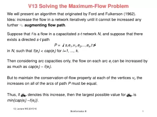
1. V12 Solving the Maximum-Flow Problem We will present an algorithm that originated by Ford and Fulkerson (1962). Idea: increase the flow in a network iteratively until it cannot be increased any further  augmenting flow path. Suppose that f is a flow in a capacitated s-t network N, and suppose that there exists a directed s-t path P = s,e1,v1,e2,...,ek,t in N, such that f(ei) < cap(ei) for i=1, ..., k. Then considering arc capacities only, the flow on each arc ei can be increased by as much as cap(ei) – f(ei). But to maintain the conservation-of-flow property at each of the vertices vi, the increases on all of the arcs of path P must be equal. Thus, if P denotes this increase, then the largest possible value for P is min{cap(ei} –f(ei)}. Bioinformatics III

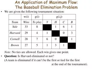
2. Solving the Maximum-Flow Problem Example: Left side: the value of the current flow is 6. Consider the directed s-t path P = s,x,w,t. The flow on each arc of path P can be increased by P = 2. The resulting flow, which has value 8, is shown on the right side. Using the directed path s,v,t, the flow can be increased to 9. The resulting flow is shown right. At this point, the flow cannot be increased any further along directed s-t paths, because each such path must either use the arc directed from s to x or from v to t. Both arcs have flow at capacity. Bioinformatics III

3. Solving the Maximum-Flow Problem However, the flow can be increased further. E.g. increase the flow on the arc from source s to vertex v by one unit, decrease the flow on the arc from w to v by one unit, and increase the flow on the arc from w to t by one unit. Bioinformatics III

4. f-Augmenting Paths Definition: An s-t quasi-path in a network N is an alternating sequence s = v0,e1,v1,...,vk-1,ek,vk = t of vertices and arcs that forms an s-t path in the underlying undirected graph of N. Terminology For a given s-t quasi-path Q = s = v0,e1,v1,...,vk-1,ek,vk = t arc ei is called a forward arc if it is directed from vertex vi-1to vertex vi and arc ei is called a backward arc if it is directed from vi to vi-1. Clearly, a directed s-t path is a quasi-path whose arcs are all forward. Example. On the s-t quasi-path shown below, arcs a and b are backward, and the three other arcs are forward. Bioinformatics III

5. f-Augmenting Paths Definition: Let f be a flow in an s-t network N. An f-augmenting path Q is an s-t quasi path in N such that the flow on each forward arc can be increased, and the flow on each backward arc can be decreased. Thus, for each arc e on an f-augmenting path Q, f(e) < cap(e), if e is a forward arc f(e) > 0 if e is a backward arc. Notation For each arc e on a given f-augmenting path Q, let e be the quantity given by Terminology The quantity e is called the slack on arc e. Its value on a forward arc is the largest possible increase in the flow, and on a backward arc, the largest possible decrease in the flow, disregarding conservation of flow. Bioinformatics III

6. f-Augmenting Paths Remark Conservation of flow requires that the change in the flow on the arcs of an augmenting flow path be of equal magnitude. Thus, the maximum allowable change in the flow on an arc of quasipath Q is Q, where Example For the example network shown below, the current flow f has value 9, and the quasi-path Q = s,v,w,t is an f-augmenting path with Q = 1. Bioinformatics III

7. flow augmentation Proposition 12.2.1 (Flow Augmentation) Let f be a flow in a network N, and let Q be an f-augmenting path with minimum slack Q on its arcs. Then the augmented flow f‘ given by is a feasible flow in network N and val(f‘) = val(f) + Q. Proof. Clearly, 0  f‘(e)  cap(e), by the definition of Q. The only vertices through which the net flow may have changed are those vertices on the augmenting path Q. Thus, to verify that f‘ satisfies conservation of flow, only the internal vertices of Q need to be checked. Bioinformatics III

8. f-Augmenting Paths For a given vertex v on augmenting path Q, the two arcs of Q that are incident on v are configured in one of four ways, as shown below. In each case, the net flow into or out of vertex v does not change, thereby preserving the conservation-of-flow property. It remains to be shown that the flow has increased by Q. The only arc incident on the source s whose flow has changed is the first arc e1 of augmenting path Q. If e1 is a forward arc, then f‘(e1) = f(e1) + Q, and if e1 is a backward arc, then f‘(e1) = f(e1) - Q. In either case, □ Bioinformatics III

9. Max-Flow Min-Cut Theorem 12.2.3 [Characterization of Maximum Flow] Let f be a flow in a network N. Then f is a maximum flow in network N if and only if there does not exist an f-augmenting path in N. Proof: Necessity () Suppose that f is a maximum flow in network N. Then by Proposition 12.2.1, there is no f-augmenting path. Proposition 12.2.1 (Flow Augmentation) Let f be a flow in a network N, and let Q be an f-augmenting path with minimum slack Q on its arcs. Then the augmented flow f‘ given by is a feasible flow in network N and val(f‘) = val(f) + Q.  assuming an f-augmenting path existed, we could construct a flow f‘ with val(f‘) > val(f) contradicting the maximality of f. Bioinformatics III

10. Max-Flow Min-Cut Sufficiency () Suppose that there does not exist an f-augmenting path in network N. Consider the collection of all quasi-paths in network N that begin with source s, and have the following property: each forward arc on the quasi-path has positive slack, and each backward arc on the quasi-path has positive flow. Let Vs be the union of the vertex-sets of these quasi-paths. Since there is no f-augmenting path, it follows that sink t  Vs. Let Vt = VN – Vs. Then Vs,Vt is an s-t cut of network N. Moreover, by definition of the sets Vsand Vt , (if the flow along these edges e were not cap(e) or 0, these edges would belong to Vs!) Hence, f is a maximum flow, by Corollary 12.1.8. □ Bioinformatics III

11. Max-Flow Min-Cut Theorem 12.2.4 [Max-Flow Min-Cut] For a given network, the value of a maximum flow is equal to the capacity of a minimum cut. Proof: The s-t cut Vs,Vtthat we just constructed in the proof of Theorem 12.2.3 (direction ) has capacity equal to the maximum flow. □ The outline of an algorithm for maximizing the flow in a network emerges from Proposition 12.2.1 and Theorem 12.2.3. Bioinformatics III

12. Finding an f-Augmenting Path The discussion of f-augmenting paths culminating in the flow-augmenting Proposition 12.2.1 provides the basis of a vertex-labeling strategy due to Ford and Fulkerson that finds an f-augmenting path, when one exists. Their labelling scheme is essentially basic tree-growing. The idea is to grow a tree of quasi-paths, each starting at source s. If the flow on each arc of these quasi-paths can be increased or decreased, according to whether that arc is forward or backward, then an f-augmenting path is obtained as soon as the sink t is labelled. Bioinformatics III

13. Finding an f-Augmenting Path A frontier arc is an arc e directed from a labeled endpoint v to an unlabeled endpoint w. For constructing an f-augmenting path, the frontier path e is allowed to be backward (directed from vertex w to vertex v), and it can be added to the tree as long as it has slack e > 0. Bioinformatics III

14. Finding an f-Augmenting Path Terminology: At any stage during tree-growing for constructing an f-augmenting path, let e be a frontier arc of tree T, with endpoints v and w. The arc e is said to be usable if, for the current flow f, either e is directed from vertex v to vertex w and f(e) < cap(e), or e is directed from vertex w to vertex v and f(e) > 0. Frontier arcs e1 and e2 are usable if f(e1) < cap(e1) and f(e2) > 0 Remark From this vertex-labeling scheme, any of the existing f-augmenting paths could result. But the efficiency of Algorithm 12.2.1 is based on being able to find „good“ augmenting paths. If the arc capacities are irrational numbers, then an algorithm using the Ford&Fulkerson labeling scheme might not terminate (strictly speaking, it would not be an algorithm). Bioinformatics III

15. Finding an f-Augmenting Path Even when flows and capacities are restricted to be integers, problems concerning efficiency still exist. E.g., if each flow augmentation were to increase the flow by only one unit, then the number of augmentations required for maximization would equal the capacity of a minimum cut. Such an algorithm would depend on the size of the arc capacities instead of on the size of the network. Bioinformatics III

16. Finding an f-Augmenting Path Example: For the network shown below, the arc from vertex v to vertex w has flow capacity 1, while the other arcs have capacity M, which could be made arbitrarily large. If the choice of the augmenting flow path at each iteration were to alternate between the directed path  s,v,w,t  and the quasi path  s,w,v,t , then the flow would increase by only one unit at each iteration. Thus, it could take as many as 2M iterations to obtain the maximum flow. Bioinformatics III

17. Finding an f-Augmenting Path Edmonds and Karp avoid these problems with this algorithm. It uses breadth-first search to find an f-augmenting path with the smallest number of arcs. Bioinformatics III

18. FFEK algorithm: Ford, Fulkerson, Edmonds, and Karp Algorithm 12.2.3 combines Algorithms 12.2.1 and 12.2.2 Bioinformatics III

19. FFEK algorithm: Ford, Fulkerson, Edmonds, and Karp Example: the figures illustrate algorithm 12.2.3. <{s, x, y, z, v}, {w, a, b, c, t}> is the s-t cut with capacity equal to the current flow, establishing optimality. Bioinformatics III

20. FFEK algorithm: Ford, Fulkerson, Edmonds, and Karp At the end of the final iteration, the two arcs from source s to vertex w and the arc directed from vertex v to sink tform the minimum cut  {s,x,y,z,v }, {w,a,b,c,t} . Neither of them is usable, i.e. the flow(e) = cap(e). This illustrates the s-t cut that was constructed in the proof of theorem 12.2.3. Bioinformatics III