Last lecture summary (SVM)
Last lecture summary (SVM). Support Vector Machine Supervised algorithm Works both as classifier (binary) regressor De facto better linear classification Two main ingrediences: maximum margin kernel functions. Maximum margin. Which line is best?.

Last lecture summary (SVM)
E N D
Presentation Transcript
Support Vector Machine • Supervised algorithm • Works both as • classifier (binary) • regressor • De facto better linear classification • Two main ingrediences: • maximum margin • kernel functions
Maximum margin Which line is best?
Define the margin of a linear classifier as the width that the boundary could be increased by before hitting a datapoint. The maximum margin linear classifier is the optimum linear classifier. This is the simplest kind of SVM (linear SVM) • Maximum margin intuitively feels safest. • Only support vectors are important. • Works very well.
The decision boundary is found by constrained quadratic optimization. • The solution is found in the form • Only points on the margin (i.e. support vectors xi) have αi > 0. Lagrange multiplier
w does not to be explicitly formed, because: • Training SVM: find the sets of the parameters αi and b. • Classification with SVM:
soft margin • Allows misclassification errors. • i.e. misclassified points are allowed to be inside the margin. • The penalty to classification errors is given by the capacity parameter C (user adjustable parameter). • Large C – a high penalty to classification errors. • Decrease in C: points move inside margin.
Kernel functions • Soft margin introduces the possibility to linearly classify the linearly non-separable data sets. • What else could be done? Can we propose an approach generating non-linear classification boundary just by extending the linear classifier machinery?
We can map the input data points from the input space to the feature space by using the appropriate mapping . • In the feature space the discriminant function becomes:
Once we decide on the mapping , the coordinates of each data point in the feature space must be calculated (from the coordinates in the input space). • However, the step of explicitly calculating the coordinates in feature space can be avoided by using kernel trick.
We know that the discriminant function is given by • In the feature space it becomes • And we define kernel function
Kernel allows to calculate the inner product directly from the coordinates in the input space. • No transformation of data points to feature space is needed.
Kernels • Linear (dot) kernel • Polynomial • simple, efficient for non-linear relationships • d – degree • Gaussian
SVM parameters • Training sets the parametersαi and b. • The SVM has another set of parameters called hyperparameters. • The soft margin constant C. • Any parameters the kernel function depends on • linear kernel – no hyperparameter (except for C) • polynomial – degree • Gaussian – width of Gaussian
Multiclass SVM • SVM is defined for binary classification. • How to predict more than two classes (multiclass)? • Simplest approach: decompose the multiclass problem into several binary problems and train several binary SVM’s.
one-versus-one approach • Train a binary SVM for any two classes from the training set • For -class problem create SVM models • Prediction: voting procedure assigns the class to be the class with the maximum votes 1/2 1/3 1/4 2/3 2/4 3/4 3 1 4 1 1 4 1
one-versus-all approach • For k-class problem train only k SVM models. • Each will be trained to predict one class (+1) vs. the rest of classes (-1) • Prediction: • Winner takes all strategy • Assign new example to the class with the largest output value . 1/rest 2/rest 3/rest 4/rest
Resources • SVM and Kernels for Comput. Biol., Ratsch et al., PLOS Comput. Biol., 4 (10), 1-10, 2008 • What is a support vector machine, W. S. Noble, Nature Biotechnology, 24 (12), 1565-1567, 2006 • A tutorial on SVM for pattern recognition, C. J. C. Burges, Data Mining and Knowledge Discovery, 2, 121-167, 1998 • A User’s Guide to Support Vector Machines, Asa Ben-Hur, Jason Weston
http://support-vector-machines.org/ • http://www.kernel-machines.org/ • http://www.support-vector.net/ • companion to the book An Introduction to Support Vector Machines by Cristianini and Shawe-Taylor • http://www.kernel-methods.net/ • companion to the book Kernel Methods for Pattern Analysis by Shawe-Taylor and Cristianini • http://www.learning-with-kernels.org/ • Several chapters on SVM from the book Learning with Kernels by Scholkopf and Smola are available from this site
Software • SVMlight – one of the most widely used SVM package. fast optimization, can handle very large datasets, very efficient implementation of the leave–one–out cross-validation, C++ code • SVMstruct - can model complex data, such as trees, sequences, or sets • LIBSVM – multiclass, weighted SVM for unbalanced data, cross-validation, automatic model selection, C++, Java
Example – Learning Phase P(Outlook=Sunny|Play=Yes) = 2/9 P(Play=Yes) = 9/14 P(Play=No) = 5/14
Example - prediction • Answer this question: “Will we play tennis given that it’s cool but sunny, humidity is high and it is blowing a strong wind?” • i.e. predicts this new instace: x’=(Outl=Sunny, Temp=Cool, Hum=High, Wind=Strong) • Good strategy is to predict arg max P(Y|cool,sunny,high,strong) where Y is Yes or No.
Example - Prediction x’=(Outl=Sunny, Temp=Cool, Hum=High, Wind=Strong) Look up tables P(Outl=Sunny|Play=No) = 3/5 P(Temp=Cool|Play=No) = 1/5 P(Hum=High|Play=No) = 4/5 P(Wind=Strong|Play=No) = 3/5 P(Play=No) = 5/14 P(Outl=Sunny|Play=Yes) = 2/9 P(Temp=Cool|Play=Yes) = 3/9 P(Hum=High|Play=Yes) = 3/9 P(Wind=Strong|Play=Yes) = 3/9 P(Play=Yes) = 9/14 P(Yes|x’): [P(Sunny|Yes)P(Cool|Yes)P(High|Yes)P(Strong|Yes)]P(Play=Yes) = 0.0053 P(No|x’): [P(Sunny|No) P(Cool|No)P(High|No)P(Strong|No)]P(Play=No) = 0.0206 Given the factP(Yes|x’) < P(No|x’), we label x’ to be “No”.
Another Application • Digit Recognition • X1,…,Xn {0,1} (Black vs. White pixels) • Y {5,6} (predict whether a digit is a 5 or a 6) Classifier 5
Bayes Rule So how do we compute posterior probability that the image represents a 5 given its pixels? Why did this help? Well, we think that we might be able to specify how features are “generated” by the class label (i.e. we will try to compute likelihood). Likelihood Prior Posterior Normalization Constant
Let’s expand this for our digit recognition task: • To classify, we’ll simply compute these two probabilities and predict based on which one is greater. • For the Bayes classifier, we need to “learn” two functions, the likelihood and the prior.
Learning prior • Let us assume training examples are generated by drawing instances at random from an unknown underlying distribution P(Y), then allow a teacher to label this example with its Y value. • A hundred independently drawn training examples will usually suffice to obtain a reasonable estimate of P(Y).
Learning likelihood • Consider the number of parameters we must estimate when Y is boolean and X is a vector of nboolean attributes. • In this case we need to estimate a set of parameters (i.e. probabilities): • index i: 2n values, index j: 2 values … 2n.2 = 2n+1, • however for any fixed j the sum over i of must be 1 2(2n - 1)
So this corresponds to twodistinct parameters for each of the distinct instances in the instance space for X. • Worse yet, to obtain reliable estimates of each of these parameters, we will need toobserve each of these distinct instances multiple times. • For example, if X is a vector containing 30boolean features, then we will need to estimate more than 3 billion parameters!
The problem with explicitly modeling P(X1,…,Xn|Y) is that there are usually way too many parameters: • We’ll run out of space. • We’ll run out of time. • And we’ll need tons of training data (which is usually not available).
The Naïve Bayes Model • The Naïve Bayes Assumption: Assume that all features are independent given the class label Y. • Equationally speaking:
Naïve Bayes Training MNIST Training Data
Naïve Bayes Training • Training in Naïve Bayes is easy: • Estimate P(Y=v) as the fraction of records with Y=v • Estimate P(Xi=u|Y=v) as the fraction of records with Y=v for which Xi=u
Naïve Bayes Training • In practice, some of these counts can be zero • Fix this by adding “virtual” counts: • This is called Smoothing.
Naïve Bayes Training For binary digits, training amounts to averaging all of the training fives together and all of the training sixes together.
Assorted remarks • What’s nice about Naïve Bayes is that it returns probabilities • These probabilities can tell us how confident the algorithm is • So… don’t throw away these probabilities! • Naïve Bayes assumption is almost never true • Still… Naïve Bayes often performs surprisingly well even when its assumptions do not hold. • Very good method in text processing.
Confusion matrix also called a contingency table TP True Positives – is positive and is classified as positive TN True Negatives – is negative and is classified as negative FPFalse Positives – is negative, but is classified as positive FN False Negatives – is positive, but is classified as negative
Accuracy Accuracy = (TP + TN) / (TP + TN + FP + FN)
Information retrieval (IR) • A query by the user – to find the documents in the database. • IR systems allow to narrow down the set of documents that are relevant to a particular problem.
documents containing what I am looking for documents not containing what I am looking for
FN TP FP TN How many of the things I consider to be true are actually true? Precision = TP / (TP + FP) How much of the true things do I find? Recall = TP / (TP + FN)
Precision • A measure of exactness • A perfect precision score of 1.0 means that every result retrieved by a search was relevant. • But says nothing about whether all relevant documents were retrieved. TP FP