ROBOT KINEMATICS
ROBOT KINEMATICS. Purpose: The purpose of this chapter is to introduce you to robot kinematics, and the concepts related to both open and closed kinematics chains. Forward kinematics is distinguished from inverse kinematics. . In particular, you will Review the concept of a kinematics chain

ROBOT KINEMATICS
E N D
Presentation Transcript
ROBOT KINEMATICS Purpose: The purpose of this chapter is to introduce you to robot kinematics, and the concepts related to both open and closed kinematics chains. Forward kinematics is distinguished from inverse kinematics.
In particular, you will • Review the concept of a kinematics chain • Distinguish serial from parallel robots structures. • Relate a robot’s degrees-of-freedom (dof) to the joint structure constraints. • Define robot redundancy. • Define serial robot types based on primary dof. • Introduce D-H coordinates. • Examine forward and inverse kinematics for serial robots. • Examine forward and inverse kinematics for parallel robots.
joint n - 1 joint 2 link i joint 1 link n link 2 joint i Fixed link 1 Kinematics chain Mechanisms can be configured as kinematics chains. The chain is closed when the ground link begins and ends the chain; otherwise, it is open.
Assuming binary pair joints (joints supporting 2 links), the degrees-of-freedom (F) of a mechanism is governed by the equation • F = l (n - 1) – • Define • F = mechanism degrees-of-freedom • n = number of mechanism links • j = number of mechanism joints • ci = number of constraints imposed by joint i • fi = degrees-of-freedom permitted by joint i • l = degrees-of-freedom in space in which mechanism functions Degrees-of-freedom (F) of a mechanism
Grubler’s criterion It is also true that l = ci + fi which leads to Grubler's Criterion: F = l (n - j - 1) + Example - 6-axis revolute robot(ABB IRB 4400): Referencing figure and using previous page equation : F = 6 (7 - 1) - 6 (5) = 6 "as expected” or by Grubler’s equation: F = 6(7 – 6 –1) + 6 (1) = 6 "as expected”
Redundant degrees-of-freedom . A redundant joint is one that is unnecessary because other joints provide the needed position and/or orientation. Can you see the redundancy among the last 3 joints on the IRB 4400?
Redundant joints can generate passive degrees-of-freedom, which must be subtracted from Grubler's equation to get F = l (n - j - 1) + - fp Redundant degrees-of-freedom A passive dof allows an intermediate link to rotate freely about an axis defined by the two joints. A passive dof cannot transfer torque.
j = 8; n = 7 L = 8 - 7 + 1 = 2 Loop Mobility Criterion The number of independent loops (L) is the total number of loops excluding the external loop. For multiple loop chains it is true that j = n + L -1 which gives Euler's equation: L = j - n + 1 The figure applies this equation for a 2 loop mechanism.
Loop Mobility Criterion Combining Euler’s equation with Grubler's Criterion, we get the Loop Mobility Criterion: å fi = F + l L
F = l (n - j - 1) + - fp S P S Dashed lines represent sameS-P-S joint combination as shown: S = spherical joint; P = prismatic joint) Parallel robots A parallel robot is a closed loop chain, whereas a serial robot is an open loop chain. A hybrid mechanism is one with both closed and open chains. The figure shows the Stewart-Gough platform. Determine the dof. Each S-P-S combination generates a passive degree-of-freedom. Thus, apply l = 6; n = 14; j1 = 6; j3 = 12; fp = 6 to get F = 6(14 - 18 -1) + (12 x 3 + 6) - 6 = 6 ....as expected!
Serial Robot Types Serial robots can be classified as revolute, spherical, cylindrical, or rectangular (translational, prismatic, or Cartesian). These classifications describe the primary DOF (degrees-of-freedom) which accomplish the global motion as opposed to the distal (final) joints that accomplish the local orientation.
Open Chain Link Coordinates According to Denavit-Hartenberg (D-H) notation (Denavit, J. and Hartenberg, "A Kinematic Notation for Lower-Pair Mechanisms Based on Matrices," J. of Applied Mechanics, June, 1955, pp. 215-221.), only four parameters (a, d, q, a) are necessary to define a frame in space (or joint axis) relative to a reference frame: z a = minimum distance between line L (the z axis of next frame) and z axis (mutually orthogonal line between line L and z axis) d = distance along z axis from z origin to minimum distance intersection point q = angle between x-z plane and plane containing z axis and minimum distance line a = angle between z axis and L . L a d a d q y x
Joint ai di qi ai Range 1 0 0 90 -90 -150 to 150 2 432 149.5 0 0 -225 to 45 3 0 0 90 90 -45 to 225 4 0 432 0 -90 -110 to 170 5 0 0 0 90 -100 to 100 6 0 55.5 0 0 -265 to 265 D-H parameters applied to Puma robot
D-H parameters and the HT Given a revolute joint a point located on the ith link can be located in i - 1 axes by the following transformation set which consist of four homogeneous transformations (2 rotations and 2 translations). The set that will accomplish this is Ai = H(d,zi-1) H(q,z i-1) H(a,xi) H(a,x i) (i = 1, ...n) Why are the D-H parameters applied as shown to generate the Ai transformation? Ai =
Other D-H Notation (used in CODE) Four parameters must be specified: ai = minimum distance between joint i axis (zi) and joint i-1 axis (zi-1) di = distance from minimum distance line (xi-1 axis) to origin of ith joint frame measured along zi axis. ai = angle between zi and zi-1 measured about previous joint frame xi-1 axis. qi = angle about zi joint axis which rotates xi-1 to xi axis in right hand sense. The xi axis is the minimum distance line defined from zi to zi+1; zi is defined as the joint rotation or translation axis axis and yi by the right hand rule (zi x xi). The origin of each joint frame is defined by the minimum distance line intersection on the joint axis.
The transformation for this set of D-H parameters is Ai = Other D-H Notation (used in CODE) What are the major differences between conventional D-H and CODE D-H?
Joint ai di qi ai Range 1 0 0 0 0 -150 to 150 2 -225 to 45 3 -45 to 225 4 -110 to 170 5 -100 to 100 6 -265 to 265 Class problem:Derive the set of CODE D-H parameters for the Puma robot being considered.
Forward Kinematics for Serial Robots Given the A transformation matrices of one joint frame relative to the preceding joint frame using conventional D-H notation, we can relate any point in the ith link to the global reference frame by the following transformation. Let vi be a point fixed to the ith link. Its coordinates ui in the global frame are (n = # dof) ui = A1 A2....Ai vi ( i = 1, 2, ... n) Typically we represent the set of transformations above by a single matrix called the T matrix Ti = A1 A2....Ai If i = n, then Tn locates the tool (or gripper) frame. We usually drop the nsubscript and simply use T.
Forward Kinematics using CODE D-H The pose of a tool frame at the end of the robot can be determined by the equation T = A1A2A3...AnG where T locates the tool relative to the robot base frame and G locates the tool relative to the last joint frame. Question: Why is G required in the CODE D-H notation, but not in the conventional D-H notation?
Inverse kinematics for serial robots Inverse kinematics raises the question: Given that I know the desired pose of the tool, what are the joint values required to move the tool to the desired pose? Forward kin: T = A1A2A3...AnG unknown known Inverse kin: A1A2A3...An= TG-1 unknown known
Inverse kinematics for Puma robot The solution, calculated in two stages, first uses a position vector from the robot base (place at waist) to the wrist. This vector allows for the solution of the first three primary DOF that accomplish the global motion. The last 3 DOF (secondary DOF) are found using the calculated values of the first 3 DOF and the orientation joint frames T4, T5, and T6 .
z 0 y 0 x 0 p 6 Inverse kinematics for Puma robot sliding y 6 approach z 6 x 6 Gripper
q = p - d6a q z 4 Yo Xo y 4 d s 6 p a x 4 n Inverse kinematics for Puma robot Let the gripper frame be defined by the unit vector triad n, s, and a, unit vectors directed along the tool’s x, y, and z axes respectively. These are specified by the known pose of the tool frame, i.e., the target frame. The origin of the 4th joint frame is determined by q and the known offset of the tool frame, d6. Zo
n = C C C C C - S S - S S C x 1 23 4 5 6 4 6 23 5 6 S - S S C C + C 6 1 4 5 6 4 Inverse kinematics for Puma robot Applying T = A1 A2....A6 and using conventional D-H notation, we multiply Ai together to get one matrix with 6 unknowns: q1, q2,..., q6. Setting the unknown terms equal to the terms of the known target frame we generate 12 equations with 6 unknown joint angles. The course notes have a full description of these equations, but the (1,1) term looks like: where C23 = cos(q2 + q3), etc.
] p q = = = = d q q q = 0 5 6 6 4 Inverse kinematics for Puma robot Since the last three joint axes intersect at a common point (concurrent axes), which is the origin of the 4th joint frame, we let q4 = q5 = q6 = 0 and also let d6 = 0 to reduce the invkin (short for inverse kinematics) equations to those of the 4th joint frame. At this point:
Inverse kinematics for Puma robot This gives the equations: qy = S1 (d4 S23 + a2 C2) + d2 C1 Remember that qx, qy, and qz are known. Is there any way that we can solve these equations for the primary joint angles q1, q2 and q3. ?
Now q1 can be determined from the qx and qy components. Let l = d4 S23 + a2 C2; thus, • qx = C1 l - d2 S1 ; qy = S1 l + d2 C1 • It can be shown that • = Solving for q1 we we get the solution: We actually apply the atan2 function using the numerator (sine) and denominator (cos) from the solution equation. Inverse kinematics for Puma robot What does this form imply?
Inverse kinematics for Puma robot How many solutions exist for q1? Explain. Can you relate these solutions to the physical configuration of the Puma robot? The solution for q3 can be found by squaring the q components adding to get cos q3 = ± sqrt[ 1 - sin2q3] q3 = tan-1 The + soln is for the elbow above hand whereas the - soln is for the elbow below hand.
a + d S - d C + q - d 2 4 3 a + d S + q - d 2 4 3 Inverse kinematics for Puma robot Now, given q3, we can expand and finally arrive at (use atan2) 2 2 2 - q ± q z 4 3 x y 2 q = tan -1 2 2 2 2 q d C - ± q z 4 3 x y 2 The - soln corresponds to the left arm configuration, + soln corresponds to right arm configuration.
Inverse kinematics for Puma robot Obviously knowing permits definition of 0T3. To determine q4, q5, and q6 we assume that an approach direction is known (a known) and that hand orientation is specified (n, s). For the PUMA robot we can arrange the joint axes such that (z4 axis direction cosines) z5 = a (z5 axis direction cosines) y6 = s (y6 axis direction cosines)
C a + S C a - S a y3 z3 y3 x3 q4 z4 q4 x3 a x4 Inverse kinematics for Puma robot Now given the above criteria, we can solve for q4 from Determine x3 and y3 from 1st and 2nd columns of 0T3 to get (use atan2) S C a - a x y 1 1 q = tan -1 4 C 1 y z 23 1 x 23 23
Inverse kinematics for Puma robot Refer to the course notes to get similar solutions for q5 and q6. How many total invkin solutions are feasible for the Puma robot? How many solutions exist in practical applications? What limits the number of invkin solutions that can be applied?
q1 q2 (x,y,z,q) q3 q3 is used to complete the tool orientation Geometric solutions for inverse kinematics
Kinematics summary: serial robots • Forward & inverse kinematics are important to robotics. • Robot teach-pendant uses direct joint control to place the robot tool at desired poses in space. • Target for an end-effector requires invkin solutions to generate the necessary joint values. • D-H parameters provide a simple way of relating joint frames to each other, although more than one D-H form proliferate the application methods. • Invkin solutions can be complex depending on the robot structure . Both analytical and geometric methods can be applied.
Forward kinematics - parallel robots • A parallel mechanism is symmetrical if the • number of limbs is equal to the number ofdegrees-of-freedom of the moving platform • joint type and joint sequence in each limb are the same • number and location of the actuated joints are the same. Otherwise, the mechanism is asymmetrical. We will examine the kinematics for symmetrical mechanisms.
Parallel robot definitions limb = a serial combination links and joints between ground and the moving rigid platform connectivity of a limb (Ck)= degrees-of-freedom associated with all joints in a limb
Observation of symmetrical mechanisms will establish that = where j is the number of joints in the parallel mechanism and m is the number of limbs. What is the connectivity of a limb of the picker robot? Note that Grubler’s Criterion does not readily apply to parallel robots because of joint redundancies. Connectivity equation Answer – 7!
Forward kinematics example The course notes present the forward kinematics solution for the Maryland (or ABB picker) robot. This solution is also found in Tsai’s text. It is complex and will not be discussed here, but you should review the solution to see how it is done. The reason for not examining this solution is found in the question: How would you use a teach pendant to program this robot?
Program picker robot? In reality you would probably not command the joints directly, but most likely command translations in the u, v, and w directions. Thus, you would not likely drive this robot using forward kinematics but only apply inverse kinematics.
p Inverse kinematics for picker robot Assume that a desired position vector p given. Find the joint angles to place point P at p. In reality, the gripper would not be located at P, but be attached to the moving platform. This is determined by gripper frame G relative to the platform coordinate axes. A target frame is specified as T. The frame for point P is determined from the fourth column of Tp = TG-1. We designate this vector as p.
Inverse kinematics for picker robot Given p we determine the location of point Ci. This is simple because the moving platform cannot rotate and thus the line between P and Ci translates only. Thus, given P (as determined by p) and the distance h, we can determine Ci as displaced from P by a vector of length h that is parallel to xi. parallel to xi Ci h P’ p P zero state xi O
Inverse kinematics for picker robot We can write a loop closure equation: AiBi + BiCi = OP + PCi – OAi and express this equation in the limb i coordinate frame (xi, yi, zi).
ci Inverse kinematics for picker robot Expressing the previous limb vector loop equation in the limb i coordinate frame, we get the matrix equations: in terms of the limb vector c shown by the green vector in the figure:
ci Inverse kinematics for picker robot The locus of motion of link BiCi is a sphere with center at Ci and radius b. From the previous matrix equation we can determine a solution for q3i as q3i = cos-1(cyi/b) P h Ci b Bi' h Bi b zi a O r xi Ai
Inverse kinematics for picker robot Given q3i we can determine an equation for q2i by summing the squares of the matrix equation to get 2ab sq3i cq2i + a2 + b2 = cxi2 + cyi2 + czi2 which leads to a solution for q2i as q2i = cos-1(k) where k = (cxi2 + cyi2 + czi2 - a2 - b2)/(2ab sq3i). Physically, we can determine two solutions for q2i ("+" angle and "-" angle similar to elbow up/down case).
Inverse kinematics for picker robot The two solutions for q1i can be determined from the matrix equation by expanding the double angle formulas, solving for the sine and cosine of q1i and then using the atan2 function to get q1i.
Inverse kinematics for picker robot An alternative solution is to sum the squares of the 1st and 3rd equations after rearranging them to this form (q3i now known): a cq1i – cxi = b sq3i c(q1i + q21) a sq1i – czi = b sq3i s(q1i + q21) leading to: cxi cq1i + czi sq1i = (a2 + cxi2+ czi2- b2 s2q3i)/(2 a) This is the familiar form we introduced earlier in the course and can be arranged to a double angle sine formula to solve for q1i , the actuation joint for each limb. This approach does not require a solution for q2i .