Mesoscale Needs for Land-Atmosphere Interaction
440 likes | 670 Vues
Mesoscale Needs for Land-Atmosphere Interaction. Paul Dirmeyer Center for Ocean-Land-Atmosphere Studies Calverton, Maryland Currently on assignment: Climate & Large-Scale Dynamics Program GEO/ATM, National Science Foundation. Outline.

Mesoscale Needs for Land-Atmosphere Interaction
E N D
Presentation Transcript
Mesoscale Needs for Land-Atmosphere Interaction Paul Dirmeyer Center for Ocean-Land-Atmosphere Studies Calverton, Maryland Currently on assignment: Climate & Large-Scale Dynamics Program GEO/ATM, National Science Foundation
Outline • Need for observations relevant to land-atmosphere interactions • Observational studies • Modeling studies • An instructive predictability/prediction study • What needs to be measured • Basic variables • Time and spatial scales • Existing networks of surface & subsurface observations • Mesonets • Climate Networks • Research Networks • Analyses, LDAS & remote sensing • CCSPO Global Water Cycle SSG white paper
Land-Climate Interaction Evap Sensible Heat Radiation Fluxes at the land surface • Simple Version 20-30% 70-80% State of the land surface Humidity Temperature Winds Soil water Vegetation Snow Albedo Roughness Soil Wetness Local circulation Large-scale dynamics Air near the surface Solar rad. Precip. Temperature Winds Vertically through the atmosphere Courtesy of J. Shukla (GMU)
FIFE Diurnal cycle composites by soil moisture Evaporative fraction LH / (LH+SH) Boundary layer depth dry wet dry wet 12 LT (Betts and Ball 1995) Net surface radiation Potential temp – specific humidity (Θ-q) wet dry dry wet Courtesy of David Lawrence (NCAR)
Processes that link L-A SHF • ECMWF reanalysis suggests strong relationships between land surface state, surface fluxes and PBL characteristics (Betts 2004 BAMS). • Q: Is this realistic? A: Yes, but free-running GCMs don’t get this (Dirmeyer et al. 2006 JHM). LHF X Axis = Soil moisture index Cloud Base PLCL Net Rad Betts (BAMS, 2004)
SHF controls PBL depth • Betts results (5-day means) suggest universality across tropics, mid- and high-latitudes. • Implies land surface state predicts cloud base (once synoptic “noise” is filtered out). Betts, BAMS, 2004
Observational Evidence Linking Planetary Boundary Layer Properties with Storm Tracks Afternoon low level flight provided continuous PBL data Turbulent Kinetic Energy Wet surface patches associated with: - weaker turbulence - lower temperatures - enhanced moisture • Positive feedback : • Storms form downstream of the “hotspots” (wet spots). • They propagate westward, this feedback propagates the hotspot westward. • The signal is strongest for 2-3 days after. • Impact diminishes as surface dries and subsequent rain events introduce new surface contrasts. Taylor et al., QJRMS, 2003. Courtesy of Jan Polcer (LMD)
Modeling studies • examining the impact of “perfectly forecasted” soil moisture on the simulation of non-extreme interannual variations... • Some examples: • Delworth and Manabe, J. Climate, 1, 523-547, 1988. • Dirmeyer, J. Climate, 13, 2900-2922, 2000. • Koster et al., J. Hydromet.,1, 26-46, 2000. • Douville et al., J. Climate, 14, 2381-2403, 2001. Observational studies go back to Namias (late ‘50s) AGCM evidence goes back to Shukla and Mintz (1982) • …or AGCM studies that only initialize the soil moisture? (i.e., studies that don’t prescribe soil moisture throughout the simulation period) • Such studies include: • Rind, Mon. Weather Rev., 110, 1487-1494, 1982. • Oglesby and Erickson, J. Climate, 2, 1362-1380, 1989. • Beljaars et al., Mon. Wea. Rev., 124, 362-383, 1996. Dry conditions Wet conditions 1987 conditions 1988 conditions
More studies... of “perfectly forecasted” soil moisture on the simulation of observed extreme events. Examples: Schubert et al. (see fig. 1 of Entekhabi et al., BAMS, 80, 2043-2058, 1999) demonstrated that their AGCM could only capture the 1988 Midwest drought and the 1993 Midwest flood if soil moistures were maintained dry and wet, respectively. Hong and Kalnay (Nature, 408, 842-844, 2000) studied the impact of dry soil moisture conditions on the maintenance of the 1998 Oklahoma-Texas drought.
Vertical Influence of Errors COLA GCM q • Sigma level where humidity MSE of land drift correction is as large as atmosphere drift correction for d46-90 (mid-Jul Aug) • Assess GCM tendency error f(x,y,z,month) for key state variables (atmosphere: T, u, v; land: SM, ST) • Create an additional forcing term in the prediction equations to counterbalance this tendency. σ Zhao et al., 2007 (in prep)
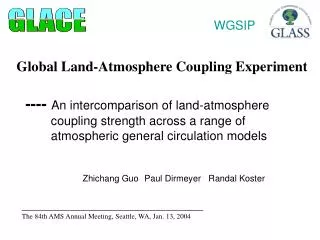
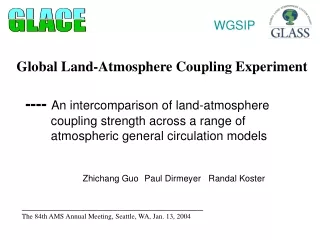
Global Land-Atmosphere Coupling Experiment The GLACE project showed that while the participating models differ in their land-atmosphere coupling strengths (the change in , or between cases S and W), certain features of the coupling patterns emerge from the models. These features are brought out by averaging over all of the model results. Koster, R. D., P. A. Dirmeyer, Z. Guo, G. Bonan, E. Chan, P. Cox, H. Davies, T. Gordon, S. Kanae, E. Kowalczyk, D. Lawrence, P. Liu, S. Lu, S. Malyshev, B. McAvaney, K. Mitchell, T. Oki, K. Oleson, A. Pitman, Y. Sud, C. Taylor, D. Verseghy, R. Vasic, Y. Xue, and T. Yamada, 2004: Regions of strong coupling between soil moisture and precipitation. Science, 305, 1138-1140.
Conventional Wisdom: Land Has a Positive Feedback on Precipitation …which affects the overlying atmospheric state (the boundary layer structure, humidity, etc.)... …causing soil moisture to increase... Precipitation wets the surface... …which causes evaporation to increase during subsequent days and weeks... …thereby inducing additional precipitation Schematically:
Observational evidence in semi-arid regimes • Niger: There is a positive correlation between daily and antecedent rainfall differences at the convective scale (~10km). 10 day differences 2-3 day differences Taylor & Lebel 1998 Courtesy of Jan Polcer (LMD)
Mechanism: ∆P ∆SM ∆E∆P Moisture limited: SM controls E Sufficient moisture: E controls SM Snow cover severs connection between SM & E Anomaly Correlation Coefficient So we can have:∆SM ∆E 99% 95% 90% – / + 90% 95% 99% Using GSWP-2 Multi-model analysis (1986-1995) Dirmeyer & Schlosser (2007 in prep).
Response curve tells why ∆SM ∆E ∆SM ∆E Evapotranspiration Soil Moisture • There is a narrow range of soil moisture where ET is very sensitive • Above that range ET controls SM • In and below that range, SM controls ET • Only in the dry range can the land surface drive the atmosphere
75 one-month ensemble forecasts (NH summer) Land initialized (right), atmosphere not Use one ensemble member as observations These “perfect model” forecasts establish upper limit of predictability An illustrative study:Land predictability and prediction Koster et al. (2004 JHM) Wind speed, humidity, air temperature, etc. from reanalysis Observed precipitation Observed radiation Mosaic LSM Initial conditions for subseasonal forecasts Regress “forecast” against “observations” to retrieve r2, the measure of forecast skill. Courtesy of Randy Koster (NASA/GSFC)
Red = high correlation Grey = where atmospheric chaos foils the forecast under assumption of perfect initialization, perfect model, and perfect validation data These results are model dependent - partial convergence among models is an indication that there is still a way to go in model development Where the land provides predictability Precipitation Temperature Courtesy of Randy Koster (NASA/GSFC)
Only where gauge density is sufficiently high and model shows sensitivity to land initial conditions could we expect impact on “real” forecasts The US appears to have the most to gain with the current observational network (note that initial conditions for land come from land data assimilation (discussed later) Initialization & validation limitations Precipitation Temperature Courtesy of Randy Koster (NASA/GSFC)
Ideal vs. actual predictability Without initialization With initialization • Validation of one month forecasts with real observations (not perfect-model). • Precipitation (top) and temperature forecasts shows positive impact, but well short of ideal. • What if we implemented a land observation network? Differences Idealized differences Without initialization With initialization Differences Idealized differences Courtesy of Randy Koster (NASA/GSFC)
Include atmosphere ICs… June r2 values, averaged over area of focus • Combination of land and atmosphere initialization gives best results • Land gives better boost for days 15-30 SSTs + land initialization + atmosphere initialization GLDAS runs: SSTs + land initialization SSTs + atmosphere initialization AMIP runs: SSTs only Warning: Statistics are based on only 15 data pairs! Courtesy of Randy Koster (NASA/GSFC)
In order to initialize the land-surface state of weather and climate forecast models, we need: Timely and stable measurements of: Soil moisture (profile) Snow (coverage, temperature and depth) Vegetation (coverage, greenness) Soil temperature (little memory, less important than others) Focus in regions of important interactions (probably biggest impact over central third of the country). QC and standardization are important for data assimilation. In order to study land-atmosphere interaction, develop models and monitor variability/change, we need: Complete observations of land surface state variables, near surface atmospheric states, and fluxes between land and atmosphere. A long enough period of record to provide a large sample that both spans the range of variability of these variables and provides for adequate statistical significance of the results. For monitoring, national distribution but less frequent sampling. What in situ obs do we need?
Time: Subsurface state variables: daily is sufficient for most applications Surface state variables: daily to hourly Fluxes: sub-hourly For operational forecasting, soil moisture is most important during the “warm season” (varies geographically); snow when snow occurs For research, long term (multi-year) data sets are a must. Field campaigns lasting only weeks can only address a limited subset of questions. Space: Heterogeneity of the land surface exists on all scales down to <1m, but scaling rules do apply. Multiple in situ measurements in the same meso-area but in different soils/vegetation needed to sample variability. Remote sensing holds promise to scale up point measurements to give a more complete 2-D picture Third dimension comes from combination of in situ profiles and models Data assimilation is the tool to bring this all together What scales of measurements?
What measurements exist now? • Mesonets • Climate Networks • Research Networks
Mesonets • Several states have mesonets • Many more are planning or building mesonets • Few include land surface measurements (e.g., OK does, KY will) • Fewer still include surface fluxes (e.g., LA has radiation) • Almost no interstate coordination
Mesonets as a backbone? • Oklahoma “invented” the mesonet, many states are implementing them, but much of the country is still uncovered. • Much variability between states, but could form the backbone of a national network. • Augmentation with soil monitoring, focused on the central third of the nation, could have best impact on forecasting. • Need interstate standards to be useful.
USDA Networks • Soil Climate Analysis Network (SCAN) monitors soil moisture and temperature SCAN Network • SNOWTEL monitors snow depth, temperature, density, etc. over western states
State climate networks (much less frequent measurements than mesonets) Agricultural focus Illinois Climate Network is nations oldest (with soil moisture) National climate networks US Climate Reference Network (FY2008 NOAA budget includes implementation of soil moisture sensors at US CRN stations for NIDIS) Other climate networks Existing Site Planned Site
ARM/CART • DOE operates the Atmospheric Radiation Measurement (ARM) program; in particular, the Southern Great Plains site consists of a Central Facility and a number of Extended Facilities Kansas Oklahoma across a large area of Oklahoma and southern Kansas (map at right - nine stations have sufficient data for comparison with the models).
Fluxnet • Mainly measure vertical fluxes of carbon and water in the lower atmosphere (also nitrogen, radiation, heat) and near-surface and surface state variables from towers. • Few include soil moisture, although the numbers are increasing. • US has most long-term sites with soil moisture measurements. • Strictly research • Frequent data quality issues
Research needs • For research purposes (understanding and model development) we need long-term, complete (surface, atmosphere and fluxes between) high-quality observations over GCM-grid or larger areas in multiple locations (duplicate the ARM-CART network in a few more locations to sample other weather/climate regimes). • Flux measurements mostly of interest for research and long-term monitoring, with some exceptions (e.g. agriculture).
GSWP-2 DVD with 10yr global 1° land-surface multi-model analysis for 50 different variables, including soil moisture and temperature at 6 levels. • Includes documentation, data (NetCDF monthly and climatological; daily for soil moisture and temperature only), sample images, and GrADS software. • Monthly data include inter-model standard deviation as well as multi-model mean. • Complete daily data online (see: www.iges.org/gswp/). Dirmeyer et al. (2005 BAMS)
Vertical and temporal structure • Daily multi-model soil wetness at 40.5°N, 89.5°W from 0-1.5m depth. • Annual cycle is evident, but there is tremendous intraseasonal and interannual variability. • Can’t rely on mean annual cycle as being representative!
Validation of multi-model analysis GSWP-2 Multi-Model Analysis ranks first 5 out of 6 times for soil moisture (total field and anomalies) – GSWP-2 models generally rank high. NCEP reanalyses are poor. Guo et al. (2006 JGR).
Land Data Assimilation Systems: Motivation • Quantification and prediction of hydrologic variability • Critical for initialization and improvement of weather/climate forecasts • Critical for applications such as floods, agriculture, military operations, etc. • Maturing of hydrologic observation and prediction tools: • Observation: Forcing, storages(states), fluxes, and parameters. • Simulation: Land process models (Hydrology, Biogeochemistry, etc.). • Assimilation: Short-term state constraints. • “LDAS” concept: • Bring state-of-the-art tools together tooperationallyobtain high quality land surface conditions and fluxes. • Optimal integration of land surface observations and predictions. • Continuous in time&space; multiple scales; retrospective, realtime, forecast Courtesy of Paul Houser (CREW/GMU)
Background: Land Surface Observations Precipitation:Remote-Sensing: SSM/I, TRMM, AMSR, GOES, AVHRR In-Situ: Surface Gages and Doppler Radar Radiation:Remote-Sensing: MODIS, GOES, AVHRR In-Situ: DOE-ARM, Mesonets, USDA-ARS Surface Temperature:Remote-Sensing: AVHRR, MODIS, SSM/I, GOES In-Situ: DOE-ARM, Mesonets, NWS-ASOS, USDA-ARS Soil Moisture:Remote-Sensing: TRMM, SSM/I, AMSR, HYDROS, ESTAR, NOHRSC, SMOS In-Situ: DOE-ARM, Mesonets, Global Soil Moisture Data Bank, USDA-ARS Groundwater:Remote-Sensing: GRACE In-Situ: Well Observations Snow Cover, Depth & Water:Remote-Sensing: AVHRR, MODIS, SSM/I, AMSR, GOES, NWCC, NOHRSC In-Situ: SNOTEL Streamflow:Remote-Sensing: Laser/Radar Altimiter In-Situ: Real-Time USGS, USDA-ARS Vegetation:Remote-Sensing: AVHRR, TM, VCL, MODIS, GOES In-Situ: Field Experiments Others: Soils, Latent & Sensible heat fluxes, etc. Courtesy of Paul Houser (CREW/GMU)
0% 20% LandData Assimilation Data Assimilation merges observations & model predictions to provide a superior state estimate. Remotely-sensed hydrologic state or storage observations (temperature, snow, soil moisture) are integrated into a hydrologic model to improve prediction, produce research-quality data sets, and to enhance understanding of complex hydrologic phenomenon. Courtesy of Paul Houser (CREW/GMU)
Remote sensing limitations • Radiation sensors (brightness temperatures) only sense the surface. This is fine for vegetation and snow coverage, skin temperature and surface moisture, but cannot directly retrieve state variables like sub-surface soil moisture, temperature, snow depth. • Most surface fluxes cannot be measured directly by remote sensing – some model algorithm must come into play. Heat fluxes (sensible & latent) are especially difficult to infer over land.
NASA’s Land Information System (LIS) WRF GCE GrADS/DODS Server LIS Coupled Uncoupled Station Data ESMF Global, Regional (Re-)Analyses or Forecasts LSM Ensemble Noah, CLM2, Mosaic, HYSSiB, VIC ESMF Satellite Products Code and Documentation at http://lis.gsfc.nasa.gov Kumar et al., (2006 EMS) Courtesy of Christa Peters-Lidard (NASA/GSFC)
WRF/GCE Ocean Models 12-Hours Ahead Atmospheric Model Forecasts LIS WRF/GCE/LIS as a NEWS Modeling Component Courtesy of Christa Peters-Lidard (NASA/GSFC) • Interoperability with standards: • The Earth System Modeling • Framework (ESMF) • Assistance for Land Modeling • Activities (ALMA) Applying this to couple LSS-SCM is straightforward. LIS Impact Example: WRF/LIS IHOP June 12, 2002 case Observed Rainfall Without LIS With LIS
Fact: Our inability to close the water/energy balances at the river basin scale crystallizes the scientific gap in our understanding of the terrestrial components of the water cycle. Models, have reached an “information limit” with poorly resolved and unmeasured processes and parameters. A platform for observing the water cycle within the “active zone” will require: integrated sensors be deployed within and over the watershed control volume and sampled such that a complete picture of the atmosphere-land surface-vegetation-subsurface couplings and feedbacks be identified, physically represented, and implemented in a new class of fully coupled models. a data management strategy should be implemented, and maintained from the outset with standardized sensor interface protocols. the initial experimental sites should be chosen to maximize the prospect of early success (e.g. extensive historical experimental and operation data and site information available). continuous, real-time observations at time scales of seconds to decades spatial measurements across scales from sub-meter to 10’s of kilometers continuous operation with two-way transmission of data and sensor control with adaptive sampling during extreme events facilities for instrument maintenance and calibration. CCSP Global Water Cycle SSG White Paper Towards an Integrated Observing Platform for the Terrestrial Water Cycle: From Bedrock to Boundary Layer Available online at: http://www.usgcrp.gov/usgcrp/ProgramElements/water.htm Courtesy of Chris Duffy (Penn State)
Requirement for research-quality measurements in the “regolith” • Possible configuration for subsurface moisture, temperature, pressure and/or level arrays. The piezometers should be installed 1-3 meter below the water table or deep enough to observe the water level through the annual cycle. The deeper center piezometer should be several meters below the shallow piezometers to evaluate deeper upward/downward flux. Courtesy of Chris Duffy (Penn State)
Conclusions • Institution of routine land surface and subsurface measurements would have tangible positive impacts for weather and climate forecasting and research (and other end users). • Evidence for the largest impacts for soil moisture on atmosphere suggests measurements needed east of the Rockies, west of the Appalachians. • A combination of continuous in situ observations, remote sensing, data assimilation and multi-model analyses will give the biggest gains for prediction, monitoring and research.