Linear Tracking
Linear Tracking. Jan-Michael Frahm COMP 256. Some slides from Welch & Bishop. Tracking . Tracking is the problem of generating an inference about the motion of an object given a sequence of images.

Linear Tracking
E N D
Presentation Transcript
Linear Tracking Jan-Michael Frahm COMP 256 Some slides from Welch & Bishop
Tracking Tracking is the problem of generating an inference about the motion of an object given a sequence of images. The key technical difficulty is maintaining an accurate representation of the posterior on object position given measurements, and doing so efficiently.
Model for tracking • Object has internal state • Capital indicates random variable • Small represents particular value • Obtained measurements in frame i are • Value of the measurement
General Steps of Tracking • Prediction: What is the next state of the object given past measurements • Data association: Which measures are relevant for the state? • Correction: Compute representation of the state from prediction and measurements.
predict correct Tracking
Independence Assumptions • Only immediate past matters • Measurements depend only on current state • Important simplifications Fortunately it doesn’t limit to much!
Linear Dynamic Models • State is linear transformed plus Gaussian noise • Relevant measures are linearly obtained from state plus Gaussian noise • Sufficient to maintain mean and standard deviation
A really simple example We are on a boat at night and lost our position • We know: • star position
Constant Velocity p is position of boat, v is velocity of boat state is We only measure position so
Marc makes a measurement Conditional Density Function , -2 0 2 4 6 8 10 12 14
Jan makes a measurement Conditional Density Function , -2 0 2 4 6 8 10 12 14
Combine measurements & variances Conditional Density Function -2 0 2 4 6 8 10 12 14 Online weighted average!
Rudolf Emil Kalman • Born 1930 in Hungary • BS and MS from MIT • PhD 1957 from Columbia • Filter developed in 1960-61 • Now retired
Kalman filter • Just some applied math. • A linear dynamic system: f(a+b) = f(a) + f(b) • Noisy data in hopefully less noisy out. • But delay is the price for filtering...
predict correct Predict Correct KF operates by • Predicting the new state and its uncertainty • Correcting with the new measurement
What is it used for? • Tracking missiles • Tracking heads/hands/drumsticks • Extracting lip motion from video • Fitting Bezier patches to point data • Lots of computer vision applications • Economics • Navigation
A really simple example We are on a boat at night and lost our position • We know: • move with constant velocity • star position
-2 0 2 4 6 8 10 12 14 But suppose we’re moving • Not all the difference is error. Some may be motion • KF can include a motion model • Estimate velocity and position
Process Model • Describes how the state changes over time • The state for the first example was scalar • The processmodel was “nothing changes” • A better model might be constant velocity motion
Measurement Model “What you see from where you are” not “Where you are from what you see”
Constant Velocity p is position of boat, v is velocity of boat state is We only measure position so
State and Error Covariance • First two moments of Gaussian process Process State (Mean) Error Covariance
The Process Model Process dynamics Uncertainty over interval State transition Difficult to determine
Measurement Model Measurement relationship to state Measurement uncertainty Measurement matrix
Predict (Time Update) a priori state, error covariance, measurement
Kalman gain Measurement Update (Correct) a posteriori state and error covariance Minimizes posteriori error covariance
The Kalman Gain Weights between prediction and measurements to posteriori error covariance For no measurement uncertainty State is deduced only from measurement
The Kalman Gain Simple univariate (scalar) example a posteriori state and error covariance
Summary PREDICT CORRECT
Estimating a Constant The state transition matrix The measurement matrix Prediction
Kalman Filter Web Site • Electronic and printed references • Book lists and recommendations • Research papers • Links to other sites • Some software • News http://www.cs.unc.edu/~welch/kalman/
Java-Based KF Learning Tool • On-line 1D simulation • Linear and non-linear • Variable dynamics http://www.cs.unc.edu/~welch/kalman/
KF Course Web Page http://www.cs.unc.edu/~tracker/ref/s2001/kalman/index.html ( http://www.cs.unc.edu/~tracker/ ) • Java-Based KF Learning Tool • KF web page
Closing Remarks • Try it! • Not too hard to understand or program • Start simple • Experiment in 1D • Make your own filter in Matlab, etc. • Note: the Kalman filter “wants to work” • Debugging can be difficult • Errors can go un-noticed
Relevant References • Azarbayejani, Ali, and Alex Pentland (1995). “Recursive Estimation of Motion, Structure, and Focal Length,” IEEE Trans. Pattern Analysis and Machine Intelligence 17(6): 562-575. • Dellaert, Frank, Sebastian Thrun, and Charles Thorpe (1998). “Jacobian Images of Super-Resolved Texture Maps for Model-Based Motion Estimation and Tracking,” IEEE Workshop on Applications of Computer Vision (WACV'98), October, Princeton, NJ, IEEE Computer Society. • http://mac-welch.cs.unc.edu/~welch/COMP256/