Graphical and Smoothing Techniques for Sequence Analysis in Social Dynamics
500 likes | 623 Vues
This work by Raffaella Piccarreta from Bocconi University explores the use of graphical tools to analyze life course sequences, focusing on identifying trends and rare trajectories. It emphasizes the importance of selecting suitable dissimilarity criteria to compare sequences effectively, enabling analysts to discover typical patterns related to classification variables. By leveraging techniques like Multidimensional Scaling (MDS), the study visually represents data in low-dimensional spaces, aiding in the interpretation of complex social integration processes.

Graphical and Smoothing Techniques for Sequence Analysis in Social Dynamics
E N D
Presentation Transcript
Graphical and smoothing techniques for sequences Raffaella Piccarreta Dept. of Decision Sciences and Dondena Centre for Social Dynamics Bocconi University, Milan - Italy
Sequence analysis Aim: describe/explorelife courses using suitable graphical tools Fundamental to get an initial impression of the most relevant tendencies in data, while not disregarding possible rare trajectories Can support the analyst in the choice of the set of tracked activities, of the calendar. Can help to individuate groups of cases with typical patterns and to explore whether these patterns are related to classification variable/s
Graphical tools In our approach, the evaluation of dissimilarities between sequences is needed, to identify sequences which are ‘similar’ , i.e. which share similar structural/salient features. • Our proposal depends upon a dissimilarity criterion (thus, we obtain informative graphs) • In selecting the dissimilarity criterion, different choices can be done by the analyst • We consider the availability of different dissimilarity criteria as an advantageous opportunity to ‘choose how to represent data’ (in a sense which will be clarified later) depending on the aim of the analysis and on the features of the data
Graphical tools: Sequence plots time Sequence/index plots (Scherer 2001). Cases on the horizontal axis, time on the vertical one. To each case a set of stacked bars is associated, with colours and lengths depending upon states and their durations. cases To avoid the confusion consequent to a random order of the cases on the horizontal axis, a suitable arrangement of sequences is needed. A possibility is to order sequences according to duration of particular activities or to age at entry in a given activity (univariate criterion). We propose instead to order sequences according to the first Multidimensional Scaling (MDS) factor (multivariate / data driven)
Multidimensional Scaling F2 12 1 2 F1 Conditionally to a dissimilarity criterion Factors are estimated which can be considered as responsible of the observed dissimilarities. MDS represents dissimilarities as distances between points of a low-dimensional space.
Multidimensional Scaling The MDS solution is usually put in so-called principal axis orientation. I.e., the MDS factors have a decreasing order of importance. Conditionally to the extraction method, the 1° factor is that explaining at best dissimilarities, the 2° factor is the next more important factor and so on. The 1st MDS factor is the one explaining at best the chosen dissimilarities: it is usually ‘based’ upon a combination of durations/ages at entry and it provides the best dissimilarity-based ordering criterion (multivariate / data driven).
The data • PSIN Data - Panel study of Social Integration in the Netherlands • 6 waves (1987, 1989, 1991, 1995, 1999/2000 and 2005/2006) • Reference: Lifbroer AC and Kalmijn M. (1997) PSIN Codebook • Focus: females’ work and school / union and family formation careers. We consider only women observed on the age span 15-34 (complete data, N = 326 / years of birth ’61 and ‘65).
The data For each woman we build, on a monthly (229 months) time scale, one sequence type representation of each career. The following activities are tracked over the considered period: School/Work: S1/S2/S3 Lower/Medium/Higher secondary education WP Part time working WF Working full time U None of the previous states (unemployment) Family N0/N1/N2/N3 No Cohabitation/Children U0/U1/U2/U3 Cohabitation with partner/Children M0/M1/M2/M3 Marriage/Children
The choice of the dissimilarity criterion A number of dissimilarity criteria are available. There are no results proving that one criterion is better than the others. Each one has appealing characteristics, from a theoretical point of view. We are not interested to compare the alternative measures or to determine which is the ‘best’. We are only concerned with the selection of a criterion assuring a reasonable ordering, the concept of ‘reasonability’ depending on the aim of the analysis.
The choice of the dissimilarity criterion Many criteria have been introduced in the literature to properly quantify the dissimilarity between sequences OMA: quantification of the effort needed to transform one sequence into another using three basic operations: insertion, deletion, substitution. Costs have to be assigned to each operation. Debate on this... Substitution costs: usually inversely proportional to the transition frequencies (otherwise set on the basis of a-priori knowledge) Indel costs: Different proposals: At least half the max substitution cost, so that substitution is preferred to two indels. More recently: Lower values ( 0.1 times the max substitution cost).
The choice of the dissimilarity criterion Many proposals to properly quantify the dissimilarity between sequences Lesnard: dynamic Hamming distance. It is based only upon substitution costs, which are related to the frequencies of the transitions from one state to another between two consecutive periods (thus varying across time). Halpin: in OMA the cost does not depend upon the length of the modified spell: costs of the operations should be weighted accordingly. The deletion of an element from a long episode produces lower costs than that of the element itself from a short episode.
The choice of the dissimilarity criterion • Elzinga. Focus is on the states sequence, i.e. the collection of visited states • The evaluation of similarity is based upon the number and/or the frequency of substructures common to two states sequences: • length of the longest common prefix (the first pattern of states, including the first visited state) • length of the longest common sub-sequences (collection of states appearing in each sequence and in the same order) • number of common sub-sequences • number of matched sub-sequences (counting how often each subsequence embedded in a states sequence can be matched with the same subsequence embedded in the other) • These measures can all be extended to account for durations. One possibility is to refer to the minimal shared time, i.e. the units of time spent in the common sub-sequences (or prefixes).
Dissimilarities • We obtained different dissimilarity matrices, using: • OMA: substitution costs based on transition frequencies and different indel costs. Similar results: only OMA05, with indel=(max substitution cost*0.5) will be presented • Lesnard Dynamic Hamming distance. Results similar to OMA, not shown. • Halpin’s OMAH • Elzinga’s criteria • Length of the longest common prefix, LCP • Number of matching sequences, NMS
Multidimensional Scaling • MDS was applied to each dissimilarity matrix • Classic/Metric MDS • Non-Metric MDS • Bayesian MDS • Using standard criteria (Stress, based upon the normalized squared distances between the observed and the reproduced dissimilarities), the Bayesian MDS solution was taken into account.
Work trajectories – MDS sequence plots OMA05 (A) and OMAH (B) provide similar (if not identical) ordering: full time workers are opposed to the unemployed. Blocks of trajectories dominated by part time work are scattered along the horizontal axes
Work trajectories – MDS sequence plots NMS (C) more focused on school, a bit more confused than OMA05 and OMAH. LCP (D) does not describe properly work careers after school. Analyticalproperties of criteria combined with the features of these careers. It is not a general consideration: for other sets of sequences focusing on the initial or the combined experienced states can provide suitable ordering
Work trajectories – MDS sequence plots For all the criteria, the appearance of the plots is influenced by short non employment or part-time work spells characterizing some trajectories. The presence of noisy sequences can make the visualisation complicated especially when the sample size increases and over-plotting becomes a more serious problem.
Graphical tools: Sequence plots Sequence plots MDS sequence plots • Even when sequences are reasonably ordered, a possible problem is the over-plottingconsequent to the limited available visual field. • As the sample size increases the thickness of the bars may become not sufficient, with a consequent difficulty to visualize individual trajectories. • In some situations individual variability (or complexity) due for example to short and non relevant spells in a state (e.g. short non employment spells between two jobs in a work history) can mask the most salient features of the trajectories. • The sequences deviating from the others can be hard to visualise and/or to individuate (also when cluster analysis is used….)
Graphical tools: Smoothed MDS Sequence plots We introduce a criterion to smooth sequences, reducing individual noise and permitting to unveil the ‘structural’ features of life courses. In our smoothed MDS sequence plots the smoothed sequences are plotted, ordered according to the first MDS factor. We propose criteria to measure the quality of the smoothing for each specific sequence, and use this information to individuate outliers sequences, possibly under-represented in the plots.
Graphical tools: Smoothed MDS Sequence plots • For each sequence, si, we focus on its neighbourhood, Ni, i.e. the set of sequences closest to si. • The original sequence si is substituted by a summary of cases in Ni, the smoothed sequence, i. • The distinction between what has to be considered as ‘structure’ and what as individual and negligible noise, depends upon the chosen dissimilarity criterion, (.,.), which plays consequently a crucial role in the definition of the Ni’s and of the smoothed sequences i’s
The smoothed sequences For given Ni and (.,.), we suggest to smooth a sequence si using the medoid of cases in Ni, that is the sequence having the minimum (total) distance from all the others: Being the most centrally located case, the medoid is a good local representative of the cases in Ni, and it can be obtained also when only dissimilarities are available
The neighborhoods • For given (.,.), possible proposals to choose Ni are: • The set of the knearest neighbours of si. • For a fixed radius, r, the set of sequences that are closer than r to si. • A combination of the two criteria: k is chosen, the maximal distance between si and its k neighbours is determined, ri, and the set of sequences closer that rito si are selected in Ni A relevant issue concerns the selection of k and/or r.
The neighborhoods A leave-one-out cross-validation procedure is used to choose k or r. To choose k, the medoid i –i ( k) is obtained without considering si. The leave-one-out cross-validation error is the sum of the dissimilarities between each original sequence and the corresponding medoid The ‘best’ value of kaccording to this criterion is that minimizing CV. A similar reasoning can be applied to select r. The described approaches select the same k (resp. r) for all the cases. If the criteria are combined, the radius is different from case to case.
The neighborhoods • A more flexible procedure combines the nearest neighbours and the radius approaches, and allows both k and r to vary across cases • For a given si, the leave-one-out cross-validation procedure is first applied to select the number of nearest neighbours, k*i. • The maximal distance between siand its k*i nearest neighbours, is determined, r*i • N*i is selected as the set of cases closer than r*i to si. • Therefore, both the number of neighbours and/or the radius are ideally peculiar to each case.
The quality of the smoothing The performance of the alternative smoothing methods can be evaluated using the prediction error, i.e., the sum of the dissimilarities between the original and the smoothed sequences. Toreason in relative rather than in absolute terms, we refer to the prediction error corresponding to the general medoid associated to the whole sample: The resulting quality criterion is: measuring the relative decrease in the prediction error when passing from the general medoid to the specific ones.
The quality of the smoothing Adopting another approach, note that the original dissimilarity between the i-th and the h-th sequence, (si , sh), is approximated by the dissimilarity between the two smoothed sequences, (i , h). The sum of the squared differences [(si , sh) – (i , h)]2 can also be used to evaluate the goodness of fit. This is a generalisation of the stress, solely used to evaluate the quality of an MDS solution. Adopting a procedure which is rather common in MDS, also in this case we consider a measure normalized using the sum of the squared original distances:
The choice of the dissimilarity criterion • In our smoothed MDS sequence plots the smoothed sequences are plotted, ordered according to their score on the first MDS factor. • The dissimilarity measure (.,.) plays consequently a double role. • First, it determines the ordering criterion. • Second, it is used to determine both the neighbours and the medoids in the smoothing procedure.
Smoothing PSIN data • Turning back to data, we will focus on the OMA05 and OMAH criteria (MDS factors extracted using the bayesian approach). • In the smoothing procedure, different definitions of neighbourhoods were considered (cross-validation procedure always used to select parameters) • Nearest Neighbours (k) • Radius (r) • Combination of k and r – with r varying across cases • Combination of k and r – both varying across cases • Using the R2 and S2 criteria introduced before, the last criterion was selected
Work trajectories Smoothed MDS sequence plots Smoothed MDS sequence plots: A) OMA05 B) OMAH 1) For each sequence its neighbourhood is determined 2) The original sequences are replaced by the neighbourhoods’ medoids 3) Medoids are ordered according to their score on the MDS factor. The ordering of cases can differ from that in the original MDS plots. Here similar medoids are plotted close one to another, improving sequences’ representation.
Work trajectories Smoothed MDS sequence plots Due to the double role (ordering / smoothing) played by dissimilarity, one can also combine criteria depending to the specific aim of the visualisation. (A) OMA05; (B) OMAH (C) Combination of OMA05 (ordering) and OMAH (smoothing). Visualisation improved, individual noise reduced, main patterns more evident. Note: the definition of ‘noise’ depends on the chosen dissimilarity criterion.
Work trajectories Smoothed MDS sequence plots We now focus on the quality of the approximation R 2(OMAH)=0.723 [R 2(OMA05)=0.847 ; R 2(NMS)=0.697] The approximation provided by the smoothed sequences is rather convenient as compared to the general medoid. Note that a low R2 can also be observed when the general medoid provides a satisfactory smoothing for the sequences Stress-based statistic: S 2(OMAH)=0.289 [S 2(OMA05)=0.117, S 2(NMS)=0.116] Some authors suggest interpreting the MDS stress informally and indicate 0.1 as the maximum value which can be considered as acceptable. In MDS the dissimilarities are reproduced based on factors which are free to vary, whilst here we focus on medoids. Hence this approximation can be considered again as satisfactory. In the following we refer to OMAH to illustrate how outliers can be identified
Misrepresented Work trajectories Smoothed MDS sequence plots An interesting characteristic of our tools is that for each sequence the dissimilarity between the original and the smoothed sequence, (i , h), can be used to determine which sequences are badly approximated. To do this, we obtain the percentiles of the (i , h)’s and flag as critical cases with a prediction error higher than the 80-th percentile. The critical sequences are compared with the smoothed ones to verify whether some ‘structural’ characteristics were masked for some trajectories.
Family trajectories Smoothed MDS sequence plots Now consider the family formation patterns. Smoothed sequences plots are presented, obtained using OMAH(A) and NMS (B). In (C) a combination of NMS (ordering) and OMAH (smoothing) is reported. Here the use of these plots is not strictly necessary: the original MDS sequence plots already provide a satisfactory representation of sequences, and over-plotting is not a serious issues. Nonetheless this example highlights the usefulness of these plots in extracting outliers
Misrepresented family trajectories Smoothed MDS sequence plots In the plots aside the poorly smoothed sequences are reported: those of women who had children alone or during a cohabitation, or experienced a relatively short period of cohabitation before marrying. The possibility to analyze critical careers is particularly important beyond the usefulness of graphical tools per se. It is also possible to analyze for each case the number of neighbours or the radius of the neighbourhood, to distinguish between sequences having dense neighbourhoods with similar cases from those which are instead more isolated
Smoothed MDS sequence plots • Visualisation of sequences focused on the most salient features • Permit to individuate poorly-represented sequences, i.e. trajectories with very peculiar characteristics. • It is possible to analyze in a detailed manner the entire ‘tail’ of the ‘extreme’ or deviating sequences. Separate plots can be considered for sequences characterized by more and more severe approximation errors. Thus, ideally one might consider a plot for prediction errors between the 60-th and the 70-th percentile, the 70-th and 80-th percentile, and so on. • Can be used to smooth and to simplify the visual representation of subgroups of cases determined, for example, using cluster analysis or classification trees. • In this case, it is also possible to inspect in details the level of cohesion of the groups, to monitor the variation in the quality of the smoothing when passing from the entire dataset to the subgroups for each case.
Cluster analysis applied to work trajectories (OMAH dissimilarity). Ward’s algorithm was used and 6 clusters selected Using smoothed MDS sequence plots
Using smoothed MDS sequence plots Clusters can be analyzed using the same approach described before: sequences ‘extraneous’ to the others in a cluster can be identified. Note that when the whole dataset is considered, for each sequence its neighbours and the smoothed sequence can be determined unconditionally. Instead, when focusing only on cases placed in the same cluster, a constrained smoothed sequence is determined. Therefore the level of overlapping between clusters can be evaluated wrt relatively unexplained trajectories
Note that the R2 for clusters will generally be lower than that for the whole sample (here, 0.72). Actually, the smoothing procedure is convenient when the general medoid does not effectively describe cases in the cluster. Thus, relatively homogeneous clusters can be expected to be characterized by lower R2 values. For hierarchically nested sub-samples it is therefore possible to evaluate the quality of achieved internal homogeneity focusing on the decrease of the R2 Using smoothed MDS sequence plots
The same analysis can be conducted to compare groups of cases induced by the levels of one (categorical) covariate. Aside, the year of birth (1961 or 1965) is taken into account. Can be implemented in the context of classification trees for sequences Using smoothed MDS sequence plots
Using smoothed MDS sequence plots We refer to data in Mc Vicar, Anyadike-Danes (2002, JRSS series A)collected on N = 712 young people from Northern Ireland. Monthly activity information is available for a period of 6 years (T = 72 months), following the completion of compulsory education. S School FE Further education HE Higher education T Training E Employment JL Joblessness The dissimilarity matrix was built using OMA, with substitution costs inversely related to the transition frequencies and indel cost equal to 1.
Using smoothed MDS sequence plots Aside are the MDS (bottom panel) and the smoothed MDS sequence plots (upper panel). Clusters of sequences were obtained using Ward’s algorithm. 6 clusters were selected
Clusters Clusters can be analyzed using the same approach described before. For example, sequences ‘extraneous’ to the others in a cluster can be identified.
Clusters Also note that when the whole dataset is considered, for each sequence its neighbours and the consequent smoothed sequence can be determined unconditionally. Instead, when focusing only on cases placed in the same cluster, a constrained smoothed sequence is determined. Therefore the level of overlapping between clusters can be evaluated wrt relatively unexplained trajectories
Clusters Also, note that the R2 characterizing clusters is generally lower than that characterizing the whole sample. This is reasonable, since the smoothing procedure is convenient when the general medoid does not effectively describe cases in the cluster. Thus, relatively homogeneous clusters can be expected to be characterized by lower values of the R2. For hierarchically nested sub-samples it is therefore possible to evaluate the quality of achieved internal homogeneity focusing on the decrease of the R2.
Note that the R2 for clusters are generally lower than that for the whole sample. Actually, the smoothing procedure is convenient when the general medoid does not effectively describe cases in the cluster. Thus, relatively homogeneous clusters can be expected to be characterized by lower R2 values. For hierarchically nested sub-samples it is therefore possible to evaluate the quality of achieved internal homogeneity focusing on the decrease of the R2. Clusters
Dissimilarities • We obtained different dissimilarity matrices, using: • OMA: substitution costs based on transition frequencies and different indel costs. Similar results: only indel=(max substitution cost*0.5) will be presented • Lesnard Dynamic Hamming distance. Results similar to OMA, not shown. • Halpin’s OMAH • Elzinga’s criteria • Length of the longest common prefix, LCP • Number of matching sequences, NMS