GRAPHICAL DESCRIPTIVE TECHNIQUES
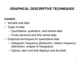
GRAPHICAL DESCRIPTIVE TECHNIQUES. Content Variable and data Types of data Quantitative, qualitative, and ranked data Cross sectional and time series data Graphical techniques for quantitative data Histogram: frequency distribution, relative frequency distribution, shapes of histograms

GRAPHICAL DESCRIPTIVE TECHNIQUES
E N D
Presentation Transcript
GRAPHICAL DESCRIPTIVE TECHNIQUES Content • Variable and data • Types of data • Quantitative, qualitative, and ranked data • Cross sectional and time series data • Graphical techniques for quantitative data • Histogram: frequency distribution, relative frequency distribution, shapes of histograms • Ogives, stem and leaf displays and dot plots
VARIABLE AND DATA • Variable • A characteristic of a population or sample that is of interest to us. • Example • In case of Hudson Auto a variable is the average cost of parts used in engine tune-ups.
VARIABLE AND DATA • Data • The actual values of the variables • Data may be quantitative, qualitative or ranked • Example • In case of Hudson Auto data are the actual costs of parts used in 50 engine tune-ups observed:
QUANTITATIVE DATA • Quantitative data may have a ratio scale • Data possessing a natural zero point and organized into measures for which differences are meaningful. • Examples: Money, income, sales, profits, losses, heights of NBA players • Quantitative data may also have an interval scale • The distance between numbers is a known, constant size, but the zero value is arbitrary. • Examples: Temperature on the Fahrenheit scale.
QUALITATIVE DATA • Qualitative data has a nominal scale • Data that can only be classified into categories and cannot be arranged in an ordering scheme. • Examples: eye color, gender, marital status, religious affiliation, etc. • Examples: Suppose that the responses to the marital-status question is recorded as follows: Single 1 Divorced 3 Married 2 Widowed 4
RANKED DATA • Ranked data has an ordinal scale • Data or categories that can be ranked; that is, one category is higher than another. However, numerical differences between data values cannot be determined. • Examples: Maclean’s ranking (medical doctoral); 1. University of Toronto 2. University of British Columbia 3. Queen’s university • Examples: Opinion survey: Excellent 4 Fair 2 Good 3 Poor 1
DISCRETE AND CONTINUOUS DATA • Discrete • Assume values that can be counted. • Example: Number of defective items, number of customers arrive in a bank • Continuous • Can assume all values between any two specific values. They are obtained by measuring. • Example: length, weight, volume
CROSS-SECTIONAL AND TIME-SERIES DATA • Cross-sectional data • Observations are measure at the same time • Examples: Marketing surveys and political opinion polls • Time-series data • Observations are measured at successive points in time • Examples: Monthly sales data, daily temperature data
HISTOGRAM Consider the following data that shows days to maturity for 40 short-term investments
HISTOGRAM • First, construct a frequency distribution • An arrangement or table that groups data into non-overlapping intervals called classes and records the number of observations in each class • Approximate number of classes: See Table 2.3, p. 29 Number of observation Number of classes Less than 50 5-7 50-200 7-9 200-500 9-10 500-1,000 10-11 1,000-5,000 11-13 5,000-50,000 13-17 More than 50,000 17-20
HISTOGRAM • Approximate class width is obtained as follows:
HISTOGRAM Classes and counts for the days-to-maturity data
HISTOGRAM • Class relative frequency is obtained as follows:
RELATIVE FREQUENCY HISTOGRAM Relative-frequency distribution for the days-to-maturity data
FREQUENCY POLYGON • A frequency polygon is a graph that displays the data by using lines that connect points plotted for frequencies at the midpoint of classes. The frequencies represent the heights of the midpoints.
OGIVECUMULATIVE RELATIVE FREQUENCY GRAPH • A cumulative relative frequency graph or ogive is a graph that represents the cumulative frequencies for the classes in a frequency distribution.
OGIVE CUMULATIVE RELATIVE FREQUENCY GRAPH 1.000 1.000 0.900 0.800 0.725 0.600 0.550 Cumulative Frequency 0.400 0.300 0.200 0.100 0.075 0.000 40 50 60 70 80 90 100 Number of Days to Maturity
STEM-AND-LEAF DISPLAY • When summarizing the data by a group frequency distribution, some information is lost. The actual values in the classes are unknown. A stem-and-leaf display offsets this loss of information. • The stem is the leading digit. • The leaf is the trailing digit.
STEM-AND-LEAF DISPLAY Diagrams for days-to-maturity data: (a) stem-and-leaf (b) ordered stem-and-leaf Stem Leaves Stem Leaves 3 3 4 4 5 5 6 6 7 7 8 8 9 9 (a) (b)
DOT PLOTS Number of times oat yields was 60 bushels = 2 (count the dots)