Numerical Descriptive Techniques
Chapter 4.4.2 explores measures of central location, focusing on key statistics like the mean, median, and mode, which summarize data distributions. The arithmetic mean calculates the average, while the median identifies the middle value in ordered data, and the mode represents the most frequent observation. This chapter also highlights the relationship between these measures and their behavior in symmetrical and skewed distributions. Furthermore, measures of variability are discussed, emphasizing their importance in understanding how data spreads around the central location.


Numerical Descriptive Techniques
E N D
Presentation Transcript
Numerical Descriptive Techniques Chapter 4
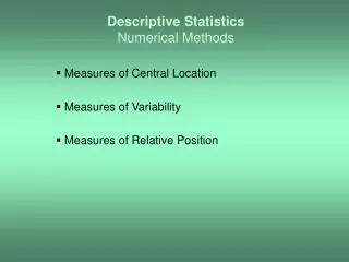
4.2 Measures of Central Location • Usually, we focus our attention on two types of measures when describing population characteristics: • Central location (e.g. average) • Variability or spread The measure of central location reflects the locations of all the actual data points.
With one data point clearly the central location is at the point itself. 4.2 Measures of Central Location • The measure of central location reflects the locations of all the actual data points. • How? With two data points, the central location should fall in the middle between them (in order to reflect the location of both of them). But if the third data point appears on the left hand-side of the midrange, it should “pull” the central location to the left.
Sum of the observations Number of observations Mean = The Arithmetic Mean • This is the most popular and useful measure of central location
The Arithmetic Mean Sample mean Population mean Sample size Population size
Example 4.2 Suppose the telephone bills of Example 2.1 represent the populationof measurements. The population mean is The arithmetic mean The Arithmetic Mean • Example 4.1 The reported time on the Internet of 10 adults are 0, 7, 12, 5, 33, 14, 8, 0, 9, 22 hours. Find the mean time on the Internet. 0 7 22 11.0 42.19 38.45 45.77 43.59
Example 4.3 Find the median of the time on the internetfor the 10 adults of example 4.1 Suppose only 9 adults were sampled (exclude, say, the longest time (33)) Comment Even number of observations 0, 0, 5, 7, 8,9, 12, 14, 22, 33 The Median • The Median of a set of observations is the value that falls in the middle when the observations are arranged in order of magnitude. Odd number of observations 8 8.5, 0, 0, 5, 7, 89, 12, 14, 22 0, 0, 5, 7, 8,9, 12, 14, 22, 33
The Mode • The Mode of a set of observations is the value that occurs most frequently. • Set of data may have one mode (or modal class), or two or more modes. For large data sets the modal class is much more relevant than a single-value mode. The modal class
The Mode The Mean, Median, Mode The Mode • Example 4.5Find the mode for the data in Example 4.1. Here are the data again: 0, 7, 12, 5, 33, 14, 8, 0, 9, 22 Solution • All observation except “0” occur once. There are two “0”. Thus, the mode is zero. • Is this a good measure of central location? • The value “0” does not reside at the center of this set(compare with the mean = 11.0 and the mode = 8.5).
Relationship among Mean, Median, and Mode • If a distribution is symmetrical, the mean, median and mode coincide • If a distribution is asymmetrical, and skewed to the left or to the right, the three measures differ. A positively skewed distribution (“skewed to the right”) Mode Mean Median
Relationship among Mean, Median, and Mode • If a distribution is symmetrical, the mean, median and mode coincide • If a distribution is non symmetrical, and skewed to the left or to the right, the three measures differ. A negatively skewed distribution (“skewed to the left”) A positively skewed distribution (“skewed to the right”) Mode Mean Mean Mode Median Median
The Geometric Mean • This is a measure of the average growth rate. • Let Ri denote the the rate of return in period i (i=1,2…,n). The geometric mean of the returns R1, R2, …,Rn is the constant Rg that produces the same terminal wealth at the end of period n as do the actual returns for the n periods.
The Geometric Mean The Geometric Mean For the given series of rate of returns the nth period return is calculated by: If the rate of return was Rg in every period, the nth period return would be calculated by: = Rg is selected such that…
4.3 Measures of variability • Measures of central location fail to tell the whole story about the distribution. • A question of interest still remains unanswered: How much are the observations spread out around the mean value?
4.3 Measures of variability Observe two hypothetical data sets: Small variability The average value provides a good representation of the observations in the data set. This data set is now changing to...
4.3 Measures of variability Observe two hypothetical data sets: Small variability The average value provides a good representation of the observations in the data set. Larger variability The same average value does not provide as good representation of the observations in the data set as before.
? ? ? The range • The range of a set of observations is the difference between the largest and smallest observations. • Its major advantage is the ease with which it can be computed. • Its major shortcoming is its failure to provide information on the dispersion of the observations between the two end points. But, how do all the observations spread out? The range cannot assist in answering this question Range Largest observation Smallest observation
This measure reflects the dispersion of all the observations • The variance of a population of size N x1, x2,…,xN whose mean is m is defined as • The variance of a sample of n observationsx1, x2, …,xn whose mean is is defined as The Variance
Sum = 0 Sum = 0 Why not use the sum of deviations? Consider two small populations: 9-10= -1 A measure of dispersion Should agrees with this observation. 11-10= +1 Can the sum of deviations Be a good measure of dispersion? The sum of deviations is zero for both populations, therefore, is not a good measure of dispersion. 8-10= -2 A 12-10= +2 8 9 10 11 12 …but measurements in B are more dispersed then those in A. The mean of both populations is 10... 4-10 = - 6 16-10 = +6 B 7-10 = -3 13-10 = +3 4 7 10 13 16
The Variance Let us calculate the variance of the two populations Why is the variance defined as the average squared deviation? Why not use the sum of squared deviations as a measure of variation instead? After all, the sum of squared deviations increases in magnitude when the variation of a data set increases!!
The Variance Let us calculate the sum of squared deviations for both data sets Which data set has a larger dispersion? Data set B is more dispersed around the mean A B 1 2 3 1 3 5
SumA = (1-2)2 +…+(1-2)2 +(3-2)2 +… +(3-2)2= 10 SumB = (1-3)2 + (5-3)2 = 8 The Variance SumA > SumB. This is inconsistent with the observation that set B is more dispersed. A B 1 3 1 2 3 5
The Variance However, when calculated on “per observation” basis (variance), the data set dispersions are properly ranked. sA2 = SumA/N = 10/5 = 2 sB2 = SumB/N = 8/2 = 4 A B 1 3 1 2 3 5
The Variance • Example 4.7 • The following sample consists of the number of jobs six students applied for: 17, 15, 23, 7, 9, 13. Finds its mean and variance • Solution
Standard Deviation • The standard deviation of a set of observations is the square root of the variance .
Standard Deviation • Example 4.8 • To examine the consistency of shots for a new innovative golf club, a golfer was asked to hit 150 shots, 75 with a currently used (7-iron) club, and 75 with the new club. • The distances were recorded. • Which 7-iron is more consistent?
The Standard Deviation Standard Deviation • Example 4.8 – solution Excel printout, from the “Descriptive Statistics” sub-menu. The innovation club is more consistent, and because the means are close, is considered a better club
Interpreting Standard Deviation • The standard deviation can be used to • compare the variability of several distributions • make a statement about the general shape of a distribution. • The empirical rule: If a sample of observations has a mound-shaped distribution, the interval
Interpreting Standard Deviation • Example 4.9A statistics practitioner wants to describe the way returns on investment are distributed. • The mean return = 10% • The standard deviation of the return = 8% • The histogram is bell shaped.
Interpreting Standard Deviation Example 4.9 – solution • The empirical rule can be applied (bell shaped histogram) • Describing the return distribution • Approximately 68% of the returns lie between 2% and 18% [10 – 1(8), 10 + 1(8)] • Approximately 95% of the returns lie between -6% and 26% [10 – 2(8), 10 + 2(8)] • Approximately 99.7% of the returns lie between -14% and 34% [10 – 3(8), 10 + 3(8)]
The Chebysheff’s Theorem • The proportion of observations in any sample that lie within k standard deviations of the mean is at least 1-1/k2 for k > 1. • This theorem is valid for any set of measurements (sample, population) of any shape!! K Interval Chebysheff Empirical Rule 1 at least 0% approximately 68% 2 at least 75% approximately 95% 3 at least 89% approximately 99.7% (1-1/12) (1-1/22) (1-1/32)
The Chebysheff’s Theorem • Example 4.10 • The annual salaries of the employees of a chain of computer stores produced a positively skewed histogram. The mean and standard deviation are $28,000 and $3,000,respectively. What can you say about the salaries at this chain? SolutionAt least 75% of the salaries lie between $22,000 and $34,000 28000 – 2(3000) 28000 + 2(3000) At least 88.9% of the salaries lie between $$19,000 and $37,000 28000 – 3(3000) 28000 + 3(3000)
The Coefficient of Variation • The coefficient of variation of a set of measurements is the standard deviation divided by the mean value. • This coefficient provides a proportionate measure of variation. A standard deviation of 10 may be perceived large when the mean value is 100, but only moderately large when the mean value is 500
Your score 4.4 Measures of Relative Standing and Box Plots • Percentile • The pth percentile of a set of measurements is the value for which • p percent of the observations are less than that value • 100(1-p) percent of all the observations are greater than that value. • Example • Suppose your score is the 60% percentile of a SAT test. Then 40% 60% of all the scores lie here
Quartiles • Commonly used percentiles • First (lower)decile = 10th percentile • First (lower) quartile, Q1, = 25th percentile • Second (middle)quartile,Q2, = 50th percentile • Third quartile, Q3, = 75th percentile • Ninth (upper)decile = 90th percentile
Quartiles • Example Find the quartiles of the following set of measurements 7, 8, 12, 17, 29, 18, 4, 27, 30, 2, 4, 10, 21, 5, 8
15 observations Quartiles • Solution Sort the observations 2, 4, 4, 5, 7, 8, 10, 12, 17, 18, 18, 21, 27, 29, 30 The first quartile At most (.25)(15) = 3.75 observations should appear below the first quartile. Check the first 3 observations on the left hand side. At most (.75)(15)=11.25 observations should appear above the first quartile. Check 11 observations on the right hand side. Comment:If the number of observations is even, two observations remain unchecked. In this case choose the midpoint between these two observations.
Location of Percentiles • Find the location of any percentile using the formula • Example 4.11 Calculate the 25th, 50th, and 75th percentile of the data in Example 4.1
0 5 Values 3.75 0 2.75 2 3 Location 1 Location Location 3 The 2.75th location Translates to the value (.75)(5 – 0) = 3.75 Location of Percentiles • Example 4.11 – solution • After sorting the data we have 0, 0, 5, 7, 8, 9, 22, 33.
Location of Percentiles • Example 4.11 – solution continued The 50th percentile is halfway between the fifth and sixth observations (in the middle between 8 and 9), that is 8.5.
Location of Percentiles • Example 4.11 – solution continued The 75th percentile is one quarter of the distance between the eighth and ninth observation that is14+.25(22 – 14) = 16. Eighth observation Ninth observation
Quartiles and Variability • Quartiles can provide an idea about the shape of a histogram Q1 Q2 Q3 Q1 Q2 Q3 Positively skewed histogram Negatively skewed histogram
Interquartile Range • This is a measure of the spread of the middle 50% of the observations • Large value indicates a large spread of the observations Interquartile range = Q3 – Q1
1.5(Q3 – Q1) 1.5(Q3 – Q1) Whisker Whisker Box Plot • This is a pictorial display that provides the main descriptive measures of the data set: • L - the largest observation • Q3 - The upper quartile • Q2 - The median • Q1 - The lower quartile • S - The smallest observation S Q1 Q2 Q3 L
Box Plot • Example 4.14 (Xm02-01) Left hand boundary = 9.275–1.5(IQR)= -104.226 Right hand boundary=84.9425+ 1.5(IQR)=198.4438 0 -104.226 9.275 198.4438 84.9425 119.63 26.905 No outliers are found
Box Plot • Additional Example - GMAT scores Create a box plot for the data regarding the GMAT scores of 200 applicants (see GMAT.XLS) 417.5 449 512 537 575 669.5 788 575+1.5(IQR) 512-1.5(IQR)
Box Plot GMAT - continued • Interpreting the box plot results • The scores range from 449 to 788. • About half the scores are smaller than 537, and about half are larger than 537. • About half the scores lie between 512 and 575. • About a quarter lies below 512 and a quarter above 575. Q1 512 Q2 537 Q3 575 449 669.5 25% 50% 25%
Box Plot GMAT - continued The histogram is positively skewed Q1 512 Q2 537 Q3 575 449 669.5 25% 50% 25% 50% 25% 25%
Box Plot • Example 4.15 (Xm04-15) • A study was organized to compare the quality of service in 5 drive through restaurants. • Interpret the results • Example 4.15 – solution • Minitab box plot