Iterative Deepening A*
360 likes | 780 Vues
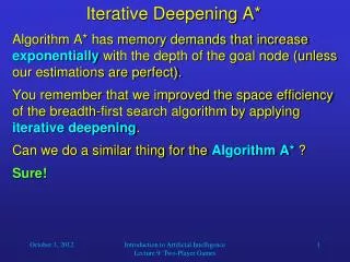
Iterative Deepening A*. Algorithm A* has memory demands that increase exponentially with the depth of the goal node (unless our estimations are perfect). You remember that we improved the space efficiency of the breadth-first search algorithm by applying iterative deepening .

Iterative Deepening A*
E N D
Presentation Transcript
Iterative Deepening A* • Algorithm A* has memory demands that increase exponentially with the depth of the goal node (unless our estimations are perfect). • You remember that we improved the space efficiency of the breadth-first search algorithm by applying iterative deepening. • Can we do a similar thing for the Algorithm A* ? • Sure! Introduction to Artificial Intelligence Lecture 9: Two-Player Games
Iterative Deepening A* • In the first iteration, we determine a “cost cut-off”f’(n0) = g’(n0) + h’(n0) = h’(n0), where n0 is the start node. • We expand nodes using the depth-first algorithm and backtrack whenever f’(n) for an expanded node n exceeds the cut-off value. • If this search does not succeed, determine the lowest f’-value among the nodes that were visited but not expanded. • Use this f’-value as the new cut-off value and do another depth-first search. • Repeat this procedure until a goal node is found. Introduction to Artificial Intelligence Lecture 9: Two-Player Games
Let us now investigate… Two-Player Games Introduction to Artificial Intelligence Lecture 9: Two-Player Games
Two-Player Games with Complete Trees • We can use search algorithms to write “intelligent” programs that play games against a human opponent. • Just consider this extremely simple (and not very exciting) game: • At the beginning of the game, there are seven coins on a table. • Player 1 makes the first move, then player 2, then player 1 again, and so on. • One move consists of removing 1, 2, or 3 coins. • The player who removes all remaining coins wins. Introduction to Artificial Intelligence Lecture 9: Two-Player Games
Two-Player Games with Complete Trees • Let us assume that the computer has the first move. Then, the game can be described as a series of decisions, where the first decision is made by the computer, the second one by the human, the third one by the computer, and so on, until all coins are gone. • The computer wants to make decisions that guarantee its victory (in this simple game). • The underlying assumption is that the human always finds the optimal move. Introduction to Artificial Intelligence Lecture 9: Two-Player Games
1 3 2 1 2 1 1 2 3 3 2 1 1 1 2 3 1 2 3 3 2 1 3 2 1 C C C 1 2 3 3 2 1 3 2 1 H H H 3 2 1 Two-Player Games with Complete Trees C 7 H 6 5 4 C 5 4 4 H 4 3 2 1 C 3 2 1 H H H H C C C Introduction to Artificial Intelligence Lecture 9: Two-Player Games
Two-Player Games with Complete Trees • So the computer will start the game by taking three coins and is guaranteed to win the game. • The most practical way of implementing such an algorithm is the Minimax procedure: • Call the two players MIN and MAX. • Mark each leaf of the search tree with 0, if it shows a victory of MIN, and with 1, if it shows a victory of MAX. • Propagate these values up the tree using the rules: • If the parent state is a MAX node, give it the maximum value among its children. • If the parent state is a MIN node, give it the minimum value among its children. Introduction to Artificial Intelligence Lecture 9: Two-Player Games
Two-Player Games with Complete Trees C 7 (min) 0 H 6 5 4 (max) 1 1 0 C 5 4 4 3 2 1 (min) 0 1 1 0 0 0 H 4 3 2 1 3 2 1 C C C 0 0 0 (max) 0 1 1 1 1 1 1 C 3 2 1 H 1 1 H 1 H H 1 H 1 H 1 (min) 0 0 0 H 0 C C 0 C 0 (max) Introduction to Artificial Intelligence Lecture 9: Two-Player Games
Two-Player Games with Complete Trees • The previous example shows how we can use the Minimax procedure to determine the computer’s best move. • It also shows how we can apply depth-first search and a variant of backtracking to prune the search tree. • Before we formalize the idea for pruning, let us move on to more interesting games. • For such games, it is impossible to check every possible sequence of moves. The computer player then only looks ahead a certain number of moves and estimates the chance of winning after each possible sequence. Introduction to Artificial Intelligence Lecture 9: Two-Player Games
Two-Player Games • Therefore, we need to define a static evaluation function e(p) that tells the computer how favorable the current game position p is from its perspective. • In other words, e(p) will assume large values if a position is likely to result in a win for the computer, and low values if it predicts its defeat. • In any given situation, the computer will make a move that guarantees a maximum value for e(p) after a certain number of moves. • For this purpose, we can use the Minimax procedure with a specific maximum search depth (ply-depth k for k moves of each player). Introduction to Artificial Intelligence Lecture 9: Two-Player Games
Two-Player Games • For example, let us consider Tic-Tac-Toe (although it would still be possible to search the complete game tree for this game). • What would be a suitable evaluation function for this game? • We could use the number of lines that are still open for the computer (X) minus the ones that are still open for its opponent (O). Introduction to Artificial Intelligence Lecture 9: Two-Player Games
Two-Player Games e(p) = 8 – 8 = 0 e(p) = 6 – 2 = 4 e(p) = 2 – 2 = 0 shows the weak-ness of this e(p) How about these? e(p) = e(p) = - Introduction to Artificial Intelligence Lecture 9: Two-Player Games
Two-Player Games Introduction to Artificial Intelligence Lecture 9: Two-Player Games
The Alpha-Beta Procedure • Now let us specify how to prune the Minimax tree in the case of a static evaluation function. • Use two variables alpha (associated with MAX nodes) and beta (associated with MIN nodes). • These variables contain the best (highest or lowest, resp.) e(p) value at a node p that has been found so far. • Notice that alpha can never decrease, and beta can never increase. Introduction to Artificial Intelligence Lecture 9: Two-Player Games
The Alpha-Beta Procedure • There are two rules for terminating search: • Search can be stopped below any MIN node having a beta value less than or equal to the alpha value of any of its MAX ancestors. • Search can be stopped below any MAX node having an alpha value greater than or equal to the beta value of any of its MIN ancestors. • Alpha-beta pruning thus expresses a relation between nodes at level n and level n+2 under which entire subtrees rooted at level n+1 can be eliminated from consideration. Introduction to Artificial Intelligence Lecture 9: Two-Player Games
The Alpha-Beta Procedure Example: max min max min Introduction to Artificial Intelligence Lecture 9: Two-Player Games
The Alpha-Beta Procedure Example: max min max min = 4 4 Introduction to Artificial Intelligence Lecture 9: Two-Player Games
The Alpha-Beta Procedure Example: max min max min = 4 5 4 Introduction to Artificial Intelligence Lecture 9: Two-Player Games
The Alpha-Beta Procedure Example: max min max = 3 min = 3 5 4 3 Introduction to Artificial Intelligence Lecture 9: Two-Player Games
The Alpha-Beta Procedure Example: max min max = 3 min = 3 = 1 5 4 3 1 Introduction to Artificial Intelligence Lecture 9: Two-Player Games
The Alpha-Beta Procedure Example: max min = 3 max = 3 min = 3 = 1 = 8 5 4 3 1 8 Introduction to Artificial Intelligence Lecture 9: Two-Player Games
The Alpha-Beta Procedure Example: max min = 3 max = 3 min = 3 = 1 = 6 5 6 4 3 1 8 Introduction to Artificial Intelligence Lecture 9: Two-Player Games
The Alpha-Beta Procedure Example: max min = 3 max = 3 = 6 min = 3 = 1 = 6 5 6 4 3 1 8 7 Introduction to Artificial Intelligence Lecture 9: Two-Player Games
The Alpha-Beta Procedure Example: = 3 max min = 3 max = 3 = 6 min = 3 = 1 = 6 5 6 4 3 1 8 7 Introduction to Artificial Intelligence Lecture 9: Two-Player Games
The Alpha-Beta Procedure Example: = 3 max Propagated from grandparent – no values below 3 can influence MAX’s decision any more. min = 3 max = 3 = 6 = 3 min = 3 = 1 = 6 = 2 5 6 2 4 3 1 8 7 Introduction to Artificial Intelligence Lecture 9: Two-Player Games
The Alpha-Beta Procedure Example: = 3 max min = 3 max = 3 = 6 = 3 min = 3 = 1 = 6 = 2 = 5 5 6 2 4 3 1 8 7 5 Introduction to Artificial Intelligence Lecture 9: Two-Player Games
The Alpha-Beta Procedure Example: = 3 max min = 3 max = 3 = 6 = 3 min = 3 = 1 = 6 = 2 = 4 5 6 4 2 4 3 1 8 7 5 Introduction to Artificial Intelligence Lecture 9: Two-Player Games
The Alpha-Beta Procedure Example: = 3 max min = 3 = 4 max = 3 = 6 = 4 min = 3 = 1 = 6 = 2 = 4 5 6 4 2 4 3 1 8 7 5 4 Introduction to Artificial Intelligence Lecture 9: Two-Player Games
The Alpha-Beta Procedure Example: = 3 max min = 3 = 4 max = 3 = 6 = 4 min = 3 = 1 = 6 = 2 = 4 = 6 5 6 4 2 4 3 1 8 7 5 4 6 Introduction to Artificial Intelligence Lecture 9: Two-Player Games
The Alpha-Beta Procedure Example: = 3 max min = 3 = 4 max = 3 = 6 = 4 min = 3 = 1 = 6 = 2 = 4 = 6 5 6 4 2 4 3 1 8 7 5 4 7 6 Introduction to Artificial Intelligence Lecture 9: Two-Player Games
The Alpha-Beta Procedure Example: = 4 max min = 3 = 4 max = 3 = 6 = 4 = 6 min = 3 = 1 = 6 = 2 = 4 = 6 5 6 4 2 4 3 1 8 7 5 4 7 6 7 Introduction to Artificial Intelligence Lecture 9: Two-Player Games
The Alpha-Beta Procedure Example: = 4 max Done! min = 3 = 4 max = 3 = 6 = 4 = 6 min = 3 = 1 = 6 = 2 = 4 = 6 5 6 4 2 4 3 1 8 7 5 4 7 6 7 Introduction to Artificial Intelligence Lecture 9: Two-Player Games