GRAPHICAL PRESENTATION AND STATISTICAL ORIENTATION

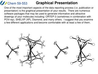
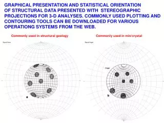
1. GRAPHICAL PRESENTATION AND STATISTICAL ORIENTATION OF STRUCTURAL DATA PRESENTED WITH STEREOGRAPHIC PROJECTIONS FOR 3-D ANALYSES. COMMONLY USED PLOTTING AND CONTOURING TOOLS CAN BE DOWNLOADED FOR VARIOUS OPERATIONG SYSTEMS FROM THE WEB. Commonly used in structural geology Commonly used in min/crystal

2. ROSE DIAGRAM, only 2-d

3. From 3 dimensions to stereogram From great circle to pole Equal area projections

4. 56 90 Great circles and poles POLE 143 PLOT PLANE 143/56 (data recorded as right-hand-rule)

5. TYPICAL STRUCTURAL DATA PLOT FROM A LOCALITY/AREA. Crowded plots may be clearer with contouring of the data. Pole to best-fit great circle to foliations Foliations Stretching lineation Shear planes

6. There are various forms of contouring, NB! notice what method you choose in the plotting program. 1% of area Common method, % = n(100)/N (N- total number of points)

7. Kamb contouring statistical significance of point concentration on equal area stereograms: binominal distribution with mean - = (NA) and standard deviation - = NA[(1-A)/NA]1/2 or /NA = [(1-A)/NA]1/2 A is chosen so that if the population has no preferred orientation, the number of points (NA) expected to fall within the counting circle is 3of the number of points (n) that actually fall within the counting circle under random sampling of the population N - number of points, A area of counting circle, if uniform distribution (NA) - expected number of points inside counting circle and [N x (1-A)] points outside the circle

8. Poles to bedding S-domain, Kvamshesten basin. NB! the contouring is different with different methods!

9. STEREOGRAM, STRUCTURAL NORDFJORD. Eclogite facies pyroxene lineation Contoured amphibolite facies foliations (Kamb contour, n=380) C) Amphibolite facies lineations

10. Rotation of data. We often want to find the orientation of pre deformation structures Determine the rotations axis Make the axis horizontal, (remember that all points must undergoes the same rotation as the axis along small circles) Rotate the desired angle (all points follow the same rotation along small circles)

11. 252 Plunging fold: 1) Determine pre-fold sedimentary lineation 2) Determine post fold lineation on western limb. Tilt fold axis horizontal (and all other points follow small-circles) Rotate around the fold axis until pole to limb P1 is horizontal. All poles rotate along small circles The original sedimentary lineation 072/00 must have been horizontal since it was formed on a horizontal bed. The original sedimentary lineation 072/00 or 252/00 Rotate P2 back to folded position around F and the lineation follows on small circle Rotate F back to EW and restore it to original Plunge, all poles follow on small circles. Restore to original orientation of axis. Lineation on western limb is found 231/09

12. Fold geometries and the stereographic projections of the folded surface

14. FOLDED LINEATIONS MAY BE USEFUL HERE TO DETERMINE FOLD MECHANISMS

16. FAULTS AND LINEATIONS STRESS INVERSION FROM FAULT AND SLICKENSIDE MEASUREMENTS “Andersonian faulting”, Mohr-Colomb fracture “law”

17. Orthorhombic faults!

18. STRESS AXES LOCATED WITH THE ASSUMPTION OF PERFECT MOHR-COLOMB FRACTURING

19. slip-linear plot SLIP-LINEAR PLOT are particularly useful for ananalyses of large fault-slip lineation data sets. Slip-lines points away from 1 towards 3 and with low concentration around 2

21. VARIOUS WAYS TO RECORD THE MEASUREMENTS IN DIFFERENT PROGRAMS

22. FAULTS WITH SLICKENSIDE AND RECORDED RELATIVE MOVEMENT FROM ONE STATION

23. SAME DATA AS BEFORE, STRESS-AXES INVERSION, RIGHT HAND SIDE ROTATED

27. Field exercises Tuesday 21/09 Departure from IF w/IF car at 09.00 am Station 1 a and b at Fornebo (small-scale fractures, veins and faults with lineations) (ca 2-3 hours) Station 2 at Nærsnes (large-scale fault between gneisses and sediments) (ca 2-3 hours) Bring food/clothes/notebook/compass/etc. Return to Blindern ca 4pm. 29/09 Report with graphical presentation of measurements