Part 5 Integration and Differentiation
560 likes | 882 Vues
Learn about numerical differentiation, numerical integration, Newton-Cotes formulas, Romberg Integration, Gauss Quadrature, Richardson Extrapolation, and more using MATLAB for symbolic computation.

Part 5 Integration and Differentiation
E N D
Presentation Transcript
Part 5 Integration and Differentiation
Part 5Numerical Differentiation and Integration • Calculus is the mathematics of change. Because engineers must continuously deal with systems and processes that change, calculus is an essential tool of engineering. • Standing in the heart of calculus are the mathematical concepts of differentiation and integration:
Slope x2, y2 y x1, y1 x
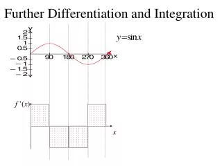
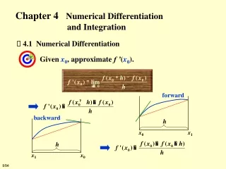
Graphical Representation of a Derivative As ∆x approaches 0 the difference approximation becomes the derivative
Part 5 Organization • Chapter 19 – Numerical Integration of Data • Newton-Cotes formulas • Chapter 20 – Numerical Integration of Functions • Romberg Integration • Gauss Quadrature • Chapter 21 – Numerical Differentiation • High Accuracy Finite Difference Approaches • Richardson Extrapolation
Chapter 19A Numerical Integration Formulas
Objectives • Understand and use single and multiple application Newton-Cotes formulas to find the integral
Methods for Differentiation and Integration • The function to be differentiated or integrated will typically be in one of the following three forms: • A simple continuous function such as polynomial, an exponential, or a trigonometric function. • A complicated continuous function that is difficult or impossible to differentiate or integrate directly. • A tabulated function where values of x and f(x) are given at a number of discrete points, as is often the case with experimental or field data.
Evaluate Analytically By Hand Using MATLAB’s Symbolic capability Approximate Methods are required Approximate Methods are required • A simple continuous function such as polynomial, an exponential, or a trigonometric function. • A complicated continuous function that is difficult or impossible to differentiate or integrate directly. • A tabulated function where values of x and f(x) are given at a number of discrete points, as is often the case with experimental or field data.
Graphical Integration • Count the number of grid squares Figure PT6_05.jpg
Graphical Integration • Strip Technique Figure PT6_06.jpg
Consider this function • Try to integrate using MATLAB’s symbolic capability
So… this won’t work!! We’ll need an approximate approach
Consider this function • Try to integrate using MATLAB’s symbolic capability • Evaluate at discrete points • Plot • Estimate the integral using the strip technique
Newton-Cotes Integration Formulas • The Newton-Cotes formulas are the most common numerical integration schemes. • They are based on the strategy of replacing a complicated function or tabulated data with an approximating function that is easy to integrate:
Approximation of an Integral based on a simple polynomial approximation A single straight line A single parabola
Approximation based on multiple application of a straight line
The Trapezoidal Rule • The Trapezoidal rule is the first of the Newton-Cotes closed integration formulas, corresponding to the case where the polynomial is first order: • The area under this first order polynomial is an estimate of the integral of f(x) between the limits of a and b: Trapezoidal rule
Error of the Trapezoidal Rule/ • When we employ the integral under a straight line segment to approximate the integral under a curve, error may be substantial: where x lies somewhere in the interval from a to b.
The Multiple Application Trapezoidal Rule/ • One way to improve the accuracy of the trapezoidal rule is to divide the integration interval from a to b into a number of segments and apply the method to each segment. • The areas of individual segments can then be added to yield the integral for the entire interval. Substituting the trapezoidal rule for each integral yields:
An error for multiple-application trapezoidal rule can be obtained by summing the individual errors for each segment: Thus, if the number of segments is doubled, the truncation error will be quartered.
Single Segment Two Segments
Single Segment Two Segments Eight Segments Eight Segments, using the built-in function
trapz • The built-in function trapz accepts an array of x and y values • They do not need to be evenly spaced
trapz • Can be used to integrate a function, by evaluating it at a number of x’s • Can be used to integrate data, even if you don’t know the function.
Chapter 19B Numerical Integration Formulas
Simpson’s Rules • More accurate estimate of an integral is obtained if a high-order polynomial is used to connect the points. The formulas that result from taking the integrals under such polynomials are called Simpson’s rules.
Simpson’s 1/3 Rule Simpson’s 1/3 Rule Resultswhen a second-order interpolating polynomial is used.
Simpson’s 3/8 Rule Results when a 3rd order interpolating polynomial is used Simpson’s 3/8 Rule
Simpson’s 1/3 Rule Single segment application of Simpson’s 1/3 rule has a truncation error of: Simpson’s 1/3 rule is more accurate than trapezoidal rule.
The Multiple-Application Simpson’s 1/3 Rule • Just as the trapezoidal rule, Simpson’s rule can be improved by dividing the integration interval into a number of segments of equal width. • Yields accurate results and considered superior to trapezoidal rule for most applications. • However, it is limited to cases where values are equispaced. • Further, it is limited to situations where there are an even number of segments and odd number of points.
Single application of the Simpson 1/3 rule Multiple application of the Simpson 1/3 rule
Simpson’s 3/8 Rule/ • An odd-segment-even-point formula used in conjunction with the 1/3 rule to permit evaluation of both even and odd numbers of segments. More accurate