Download

1 / 4
40 likes | 165 Vues
This article explains the characteristics of the graph of the reciprocal function, illustrating its symmetry and behavior at key points. We examine how the original function's zeroes translate to asymptotes in the reciprocal graph and discuss the significance of points where the original function equals +1 or -1. The vertex shifts from the original function to the reciprocal, with clear implications near key x-values. A step-by-step look into how x-values affect y-values enables a deeper understanding of the reciprocal function’s graph.

E N D
= - - 2 y ( x 2 ) 1 . 5 1 = y - - 2 ( x 2 ) 1 . 5 Y Whenever the original function is 0 the reciprocal will be undefined so we need asymptotes where the graph crosses the x-axis Whenever the original function is +1 or –1 the reciprocal will be also be +1 or –1 so we can put points on the original graph where the y-co-ord is +1 or –1. Also the vertex is at (2, – 1.5) so the “vertex” of the reciprocal will be at (2, – 0.67) If x > 3.2 For the original: x + y + For the reciprocal: x + y + 0 For the original: x 3.2then y + 0 For the reciprocal: x 3.2y + If x < 0.8 For the original: x – y + For the reciprocal: x – y + 0 For the original: x 0.8then y + 0 For the reciprocal: x 0.8y + 10 5 If 0.8 < x < 3.2 For the original: x 0.8then y – 0 For the reciprocal: x 0.8then y – For the original: x 3.2then y – 0 For the reciprocal: x 3.2then y – X -2 -1 1 2 3 4 5 -5 -10
Your turn … This time you explain why the graph of the reciprocal looks the way that it does!
= - - 2 y ( x 2 ) 1 . 5 1 = y - - 2 ( x 2 ) 1 . 5 Y 10 5 X -2 -1 1 2 3 4 5 -5 -10