Introduction to Graph drawing

1. Introduction to Graph drawing Fall 2010 Battista, G. D., Eades, P., Tamassia, R., and Tollis, I. G. 1998 Graph Drawing: Algorithms for the Visualization of Graphs. 1st. Prentice Hall PTR.

2. Constraints Henry, T.S, and Hudson, S.E. : Interactive Graph Layout. University of Arizona, Tucson, AZ, USA. UMI Order No. GAX92-25193.,1992. Dwyer, T. and Robertson, G. Layout with Circular and Other Non-linear Constraints Using Procrustes Projection. Microsoft Research, Redmond, USA. Graph Drawing , Volume 5849/2010.

3. Why using constraints? • Maximize display symmetry • Avoid edge crossings • Avoid edge bending • Keep edge length uniform • Distribute vertices uniformly

4. Constraints that are usually used • Center • Place a given vertex to the center of the drawing • External • Place a given subset of vertices on the outer boundary of the drawing • Cluster • Place a given subset of vertices close together • Left-right (top-bottom) • Draw a given path horizontally from left to right (vertically from top to bottom) • Shape • Draw a given subgraph with a predefined shape

5. Constraints that can be handled by FD-methods • Position constraints • Fixed-subgraph constraints • Constraints that can be expressed by forces or energy functions http://www.ul.ie/gd2005/contest.htm

6. Position constraints • A single point • A vertex can be nail down at a specific location • A horizontal line • A group of vertices can be arranged on a layer • A circle • A group of vertices can be restricted to a specific region Vertical and horizontal magnetic field Radial magnetic field

7. Fixed-subgraph constraints • Assign prescribed drawing to a subgraph . • May be translated or rotated, but not deformed. • Considering the subgraph as a rigid body.

8. Constraints expressed by forces • Orientation of directed edges: magnetic spring • Geometric clustering of special set of vertices • Alignment of vertices • Clustering can be achieved • For each set C of vertices, add a dummy attractor vertex vC • Add attractive forces between an attractor vC and each vertex in C. • Add repulsive forces between pairs of attractors and between attractors and vertices not in any cluster.

9. What to consider • The best layout depends on what information the user currently focused on. •  Overall layout or substructures •  User control the layout process • Large graphs • One possible solution is to build lots of graphs each of which focuses on a few substructures that the user thinks are important

10. Concepts of building interactive graph layout • An architecture for building a new simple graph layout algorithms from existing algorithms. • Parameterize graph layout algorithms to give the user control over the layout process • A high interactive mechanism for selecting portions of the graph that match the user’s current focus. Henry, T.S, and Hudson, S.E. : Interactive Graph Layout. University of Arizona, Tucson, AZ, USA. UMI Order No. GAX92-25193.,1992.

11. Composing graph layout algorithms hierarchically • Allows users to create simple new layout algorithms by plugging together existing layout algorithms. • Following the divide-and-conquer algorithm, subdivide graph into subgraphs. • Each subgraph laid out separately using the same algorithm. • Individual layouts paste together to create total graph layout.

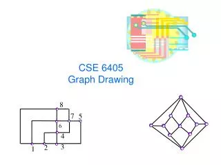
12. 2 • Placing the nodes on the perimeter of a circle • Both should be available to user • Freedom to alternate between them • Power to create new layouts 3 4 1 Eight nodes connected graph

13. Emphasizes the two shortest paths between start and destination • Row algorithm • Connections between the paths and the rest of the graph. • Concentric rings

14. Parameterized layout algorithm • Changing the root node can change the graph and focus of the layout to reflect the user's interest • Different views of the same graph with different parameterization of the same algorithm

15. Which set of nodes will produce the best subgraph? • It should be easy and fast to iteratively try different parameterization sets. • Users can discover new aspects while exploring different parameterizations. • What if user can combine the last two mechanisms? • User can customize portions of the graph by changing the parameters to the algorithm for that portion.

16. Subgraph selection • Selecting pieces that are small enough to look and focus • Apply a layout algorithm to each subgraph • Creating different views of graph until it meets the users needs • The process should be easy or it will interfere with the exploration

17. Types of selection • Manual selection • Select nodes in the graph by pointing at them with mouse, or group them with drawing rectangle around them. • For few number of nodes, or nodes that are positioned close to each other. • Algorithmic selection • Traverse the graph marking nodes as being selected • For nodes that may not be visible, or are spread through the graph.

18. Nodes root and destination manually selected . • Applying shortest path selection algorithm, which is parameterized with two nodes, selects all the nodes on the shortest path between them. • The selected nodes have been laid out by the row layout algorithm highlighting the shortest path.

19. Downward-pointing edge constraints Dwyer, T., Koren, Y., Marriott, K.: IPSep-CoLa: an incremental procedure for separation constraint layout of graphs. IEEE Transactions on Visualization and Computer Graphics 12(5), 821–828 (2006)

20. Page-boundary constraints Dwyer, T., Koren, Y., Marriott, K.: IPSep-CoLa: an incremental procedure for separation constraint layout of graphs. IEEE Transactions on Visualization and Computer Graphics 12(5), 821–828 (2006)

21. Non-overlap constraints Dwyer, T., Koren, Y., Marriott, K.: IPSep-CoLa: an incremental procedure for separation constraint layout of graphs. IEEE Transactions on Visualization and Computer Graphics 12(5), 821–828 (2006)

22. Alignment constraints Dwyer, T., Koren, Y., Marriott, K.: IPSep-CoLa: an incremental procedure for separation constraint layout of graphs. IEEE Transactions on Visualization and Computer Graphics 12(5), 821–828 (2006)

23. Constraint projection techniques • Projecting the variables: x=(x1,…,xn) with starting positions d=(d1,…,dn) against a set of constraints that define a feasible region S means finding the point x in S closest to d:

24. w2 w1 (w1+w2) x1+ ≤ x2 2 h2 (x2,y2) (x1,y1) (h2+h3) y3+ ≤ y2 h3 (x3,y3) 2 Separation constraint projection • Separation constraints: x1+d ≤ x2 , y1+d ≤ y2can be used with force-directedlayoutto impose certain spacing requirements Dwyer, T. and Robertson, G. Layout with Circular and Other Non-linear Constraints Using Procrustes Projection. Microsoft Research, Redmond, USA. Graph Drawing , Volume 5849/2010.

25. Procrustes projection • X be set of 2D points, and Y is a set of projections of X • Y has a rigid shape but can be scaled by the factor s, translated be a factor t or rotated by an orthogonal matrix T • Such that (1)

26. By differentiating with respect to t: • Substituting (2) for t in (1), • Substituting (2) and (3) in (1): T is invariant to s or t. (2) (3) What is trY’Y?

27. What is T? • It can be shown that: T=QP’, wheresvd(X’Y)=PΦQ’ is the optimal rotation Lets say we have The singular value decomposition of A, or:

28. Project X on Y • Input: matrix X of n pints, a matrix Y of n points the target configuration (centered on the origin), • Output: the projection of X on the optimally transformed Y