Download

1 / 46
870 likes | 2.1k Vues
CHAPTER ONE Principles of Mass Transfer. Mass Transfer. Introduction. Mass transfer occurs when a component in a mixture migrates in the same phase or from phase to phase because of a different in concentration between two point.

E N D
Introduction • Mass transfer occurs when a component in a mixture migrates in the same phase or from phase to phase because of a different in concentration between two point. • Somewhat similar to heat conduction, but in conduction the medium is stationary and only energy in the form of heat is being transferred. • Example of mass transfer • Evaporation of water in the open pail to the atmosphere • Coffee dissolve in water • Oxygen dissolved in the solution to the microorganism in the fermentation process • Possible driving force for mass transfer • Concentration different • Pressure different • Electrical gradient, etc
Type of Mass Transfer • Molecular diffusion • Transfer of individual molecules through a fluid by random movement from high concentration to low concentration • E.g. coffee dissolve in water in making coffee • Convective mass transfer • Using mechanical force or action to increase the rate of molecular diffusion • E,g stirred the water to dissolve coffee during coffee making
Molecular Diffusion • Diffusion of molecules when the bulk fluid is stationary given by Fick’s law c : total conc. of A and B (kgmol A+B/ m3) xA : mole fraction of A DAB :molecular diffusivity of A in B (m2/s) • If total conc., c is constant and cA=xAc, then:
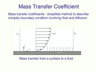
Convection Mass Transfer • When a fluid flowing outside a solid surface in forced convection motion, rate of convective mass transfer is given by: kc : mass transfer coefficient (m/s) cL1 : bulk fluid conc. cLi : conc. of fluid near the solid surface • kcdepend on: • System geometry • Fluid properties • Flow velocity
Introduction Equimolar counter diffusion Diffusion of gases A and B plus convection Gas A diffusing through stagnant, non-diffusing B Diffusion through varying cross sectional area Diffusion coefficient for gases Contents:
Fick’s Law for Gases • Molecular diffusion from cA1 to cA2 from z1 to z2 • For ideal gas PV=nRT, where c=n/V=P/RT
Equimolar Counter Diffusion PA1 > PA2 PB2 > PB1 Fig. 6.2-1
EXAMPLE 6.2-1.EquimolarCounterdiffusion Ammonia gas (A) is diffusing through a uniform tube 0.10 m long containing N2 gas (B) at 1.0132 x 10⁵ Pa pressure and 298 K. The diagram is similar to Fig. 6.2-1 in lecture. At point 1, pA1 = 1.013 x 10⁴ Pa and at point 2, pA2 = 0.507 x 10⁴ Pa. The diffusivity DAB = 0.230 x 10⁻⁴ m2/s. Calculate the flux at steady state. Repeat for Solution: Equation (6.1-13) can be used, where P = 1.0132 x 10⁵ Pa, z2 - z1 = 0.10 m, and T = 298 K. Substituting into Eq. (6.1-13) for part (a), Rewriting Eq. (6.1-13) for component B for part (b) and noting that pB1 = P - pA1 = 1.0132 x 10⁵ - 1.013 x 104 = 9.119 x 10⁴ Pa and pB2 = P - pA2 = 1.0132 x 10⁵ - 0.507 x 104 = 9.625 x 10⁴ Pa, The negative value for means the flux goes from point 2 to point 1
vA vAd vm Diffusion of Gases A and B Plus Convection1/2 vA = velocity of A relative to stationary point vAd = diffusion of A relative to moving fluid vm = molar average velocity of whole fluid or convective velocity vA = vAd + vm Multiply by cA cAvA= cAvAd + cAvm cAvA = NA = total flux of A relative to stationary point cAvAd= JA*= diffusion flux relative to moving fluid cAvm = convective flux of A relative to stationary point NA= JA* + cAvm
Diffusion of Gases A and B Plus Convection2/2 • Let N is total convective flux of the whole stream relative to stationary point; N=NA + NB = cvm or vm = (NA + NB) / c General equation become: or or If counter diffusion, the convective term become zero; NA = JA*
Gas A Diffusing Through Stagnant, Nondiffusing B1/2 • One boundary at the end of the diffusion path is impermeable to component B ( NB=0) • Evaporation of pure liquid such as benzene (A) at the bottom of narrow tube , where a large amount of air (B) passed over the top • Benzene vapor (A) diffuse through the air (B) in the tube • But at point 1, air (B) is insoluble in liquid benzene (NB=0) • Also at point 2, pA2=0 since a large volume of air is passing through • Absorption of NH3 (A) by water, which NH3 contain in air (B) • Water surface is impermeable to air (B) (NB=0) but NH3 can dissolve in water
Gas A Diffusing Through Stagnant, Non-diffusing B 2/2 • General equation • Another form to write the eq is using pBM; also we know that P = pA1 + pB1= pA2 + pB2 Time for evaporation
EXAMPLE 6.2-2. 1/2Diffusion of Water Through Stagnant, Nondiffusing Air Water in the bottom of a narrow metal tube is held at a constant temperature of 293 K. The total pressure of air (assumed dry) is 1.01325 x 10⁵ Pa (1.0 atm) and the temperature is 293 K (20°C). Water evaporates and diffuses through the air in the tube, and the diffusion path z2 - z1 is 0.1524 m (0.5 ft) long. The diagram is similar to Fig. 6.2-2a. Calculate the rate of evaporation at steady state in lb mol/h · ft2 and kg mol/s · m2. The diffusivity of water vapor at 293 K and 1 atm pressure is 0.250 x 10⁻⁴ m2/s. Assume that the system is isothermal. Use SI and English units. Solution: The diffusivity is converted to ft2/h by using the conversion factor from Appendix A.1: From Appendix A.2 the vapor pressure of water at 20°C is 17.54 mm Hg , or pA1 = 17.54/760 = 0.0231 atm = 0.0231(1.01325 x 10⁵) = 2.341 x 10³ Pa pA2 = 0 (pure air).
EXAMPLE 6.2-2. 2/2 Since the temperature is 20°C (68°F), T = 460 + 68 = 528°R = 293 K. From Appendix A.1, R = 0.730 ft3 · atm/lb · mol·°R. To calculate the value of pBM from Eq. (6.2-21), Since pB1 is close to pB2, the linear mean (pB1 + pB2)/2 could be used and would be very close to pBM. Substituting into Eq. (6.2-22) with z2 - z1 = 0.5 ft (0.1524 m),
Diffusion Through Varying Cross Sectional Area Diffusion from a sphere • Example • Evaporation of a drop of liquid • Evaporation of ball of naphthalene • Simplified eq. if (pA1<<P; pBM≈P; 2r1=D1; cA1=pA1/RT) • Time for evaporation Diffusion rate (kgmol/s)
Diffusion Coefficient for Gases1/2 Empirical equation for DAB • Chapman& Enskog P = absolute pressure in atm σAB = average collision diameter ΩD,AB = collision integral based on Lennard-Jones potential; is a ratio giving the deviation of a gas with interaction as compared to a gas rigid, elastic spheres.
Diffusion Coefficient for Gases2/2 • Fuller et al. T, in K, P in atm, n in m3 Use atomic diffusion volume (n) from Table 6.2-2. Equation 6.2-45
EXAMPLE 6.2-5. Estimation of Diffusivity of a Gas Mixture Normal butanol (A) is diffusing through air (B) at 1 atm abs. Using the Fuller et al. method, estimate the diffusivity DAB for the following temperatures and compare with the experimental data: a) For 0°C. b)For 25.9°C. c) For 0°C and 2.0 atm abs. Solution: For part (a), P = 1.00 atm,T = 273 + 0 = 273 K, MA(butanol) = 74.1, MB(air) = 29. From Table 6.2-2, Substituting into Eq. (6.2-45), This value deviates by +10% from the experimental value of 7.03 x 10⁻⁶ m2/s from Table 6.2-1. For part (b), T = 273 + 25.9 = 298.9. Substituting into Eq. (6.2-45), DAB = 9.05 x 10⁻⁶ m2/s. This value deviates by +4% from the experimental value of 8.70 x 10⁻⁶ m2/s. For part (c), the total pressure P = 2.0 atm. Using the value predicted in part (a) and correcting for pressure,
Introduction • Typical phenomena of molecular diffusion in liquids • Liquid-liquid extraction • Gas absorption • Diffusion of salts in blood • Oxygenation of river, and etc • Molecular diffusion in liquid is smaller than molecular diffusion in gases • Reason: molecules in liquid are close together compared to molecules in gases; molecules of diffusing solute will collide more frequently with liquid molecules • Diffusivity in liquid dependent on the concentration of diffusing solute.
Equimolar Counter Diffusion • Concentration is not constant, take average concentration, cav 1 and 2 represent a position/point M – average molecular weight
Average Molecular Weight Recall for average molecular weight: yi – mole fraction xi – mass fraction Don’t confuse about the symbol use for determine ave Mw. Using above eq. xA is for mass fraction and yA is for mole fraction. However, for previous molecular diffusion, xA is stand for mole fraction.
Diffusion of A through Nondiffusing B • Example: • Dilute solution of propionic acid (A) in a water (B) solution being contact with toluene • Only propionic acid (A) diffuses through the water phase, to the boundary and then into the toluene phase • Water (B) cannot diffuse in toluene-water interface
EXAMPLE 6.3-1. Diffusion of Ethanol (A) Through Water (B) 1/2 An ethanol (A)–water (B) solution in the form of a stagnant film 2.0 mm thick at 293 K is in contact at one surface with an organic solvent in which ethanol is soluble and water is insoluble. Hence, NB = 0. At point 1 the concentration of ethanol is 16.8 wt % and the solution density is ρ1 = 972.8 kg/m3. At point 2 the concentration of ethanol is 6.8 wt % and ρ2 = 988.1 kg/m3. The diffusivity of ethanol is 0.740 x 10⁻⁹ m2/s . Calculate the steady-state flux NA. Solution: The diffusivity is DAB = 0.740 x 10⁻⁹ m2/s. The molecular weights of A and B are MA = 46.05 and MB = 18.02. For a wt % of 6.8, the mole fraction of ethanol (A) is as follows when using 100 kg of solution: Then xB2 = 1 - 0.0277 = 0.9723. Calculating xA1 in a similar manner, xA1 = 0.0732 and xB1 = 1 - 0.0732 = 0.9268. To calculate the molecular weight M2 at point 2,
EXAMPLE 6.3-12/2 • Similarly, M1 = 20.07. • From Eq. (6.3-2), • To calculate xBM from Eq. (6.3-4), we can use the linear mean since xB1 and xB2 are close to each other: • Substituting into Eq. (6.3-3) and solving,
Diffusivity in Liquids • Experimental determination of diffusivity • Experimental liquid diffusivity data (Table 6.3-1) • Predictian of diffusivity in liquids a) Stokes- Einstein equation B) Wilke-Chang equation
Table 6.3-1. Diffusion Coefficients for Dilute Liquid Solutions
Stokes- Einstein Equation T- temperature in Kelvin VA- solute molar volume at normal boiling point (m3/kgmol) Table 6.3-2 m- viscosity of solution in Pa · s or kg/m · s DAB- Diffusion Coefficient in m2/s This equation holds for: -molecule with MW >1000 -molar vol ~ 0.5m3/kg mol
Wilke-Chang Equation • Solute A is dilute in the solvent B • Limited to VA (solute molar volume ) < 0.5 m3/kgmol • If solute A is water, multiply the equation by (1/2.3) where mB is in Pa.s, T in K, DAB in m2/s • Value for association parameter, Φ Water = 2.6 MeOH = 1.9 EtOH = 1.5 Benzene = 1.0 Ether = 1.0 Heptane = 1.0
EXAMPLE 6.3-2. Prediction of Liquid Diffusivity Predict the diffusion coefficient of acetone (CH3COCH3) in water at 25° and 50°C using the Wilke–Chang equation. The experimental value is 1.28 x 10⁻⁹ m2/s at 25°C (298 K). Solution: From Appendix A.2 the viscosity of water at 25.0°C is μB = 0.8937 x 10⁻³ Pas and at 50°C, 0.5494 x 10⁻³. From Table 6.3-2 for CH3COCH3 with 3 carbons + 6 hydrogens + 1 oxygen, For water the association parameter φ = 2.6 and MB = 18.02 kg mass/kg mol. For 25°C, T = 298 K. Substituting into Eq. (6.3-9), For 50°C or T = 323 K,
Introduction • Diffusion of solute in solid is slower than diffusion of solute in liquid and gases • Example application: • Leaching of food • Drying of timber, salt, food, etc. • Catalytic reaction in solid catalyst • Separation of fluid by membrane • Diffusion solute in solids can be categorized into two group • Diffusion which follow Fick’s law and does not depend on the actual structure of the solid • Diffusion in porous solids which is depend on the actual structure and void structure of the solid
Diffusion occur when the fluid or solute diffusing dissolve in the solid to form a more or less homogeneous solution Diffusion in Solids which Follow Fick’s Law and Does Not Depend on The Structure of Solids1/4 Diffusion in Solid DAB ≠ DBA Neglect convective term and assume constant concentration r1: inner radius r2: outer radius (diffusion radially through a cylinder wall of inner radius r1 and outer r2 and length L,)
Diffusion in Solids which Follow Fick’s Law and Does Not Depend on The Structure of Solids2/4 • Sometimes flux can be expressed in term of solubility (S) S= m3 (STP) /m3 solid. atm SI units S= cm3 (STP) /cm3 solid. atm cgs units • Relation between solubility and concentration SI unit cgs unit Equation for flux: (SI unit), (PA in atm)
Diffusion in Solids which Follow Fick’s Law and Does Not Depend on The Structure of Solids3/4 • Many data in literature do not determine NA in term of the value of DAB and S , but more often in term of permeability, PM • Then the flux is expressed as: • Several unit for PM in literature PM = DABS PM=m3(STP)/(s.m2.atm/m) SI unit PM=10-4 P’M P’M= cm3(STP)/(s.cm2.atm/cm) cgs unit PM=7.60 x 10⁻⁴P’’M P”M= cm3(STP)/(s.cm2.cmHg/mm)
Diffusion in Solids which Follow Fick’s Law and Does Not Depend on The Structure of Solids4/4 • When several layer solid 1,2,3…..in series and L1,L2,L3…represent thickness, flux for diffusion in solid is:
EXAMPLE 6.5-1. Diffusion of H2 Through Neoprene Membrane The gas hydrogen at 17°C and 0.010 atm partial pressure is diffusing through a membrane of vulcanized neoprene rubber 0.5 mm thick. The pressure of H2 on the other side of the neoprene is zero. Calculate the steady-state flux, assuming that the only resistance to diffusion is in the membrane. The solubility S of H2 gas in neoprene at 17°C is 0.051 m3 (at STP of 0°C and 1 atm)/m3 solid · atm and the diffusivity DAB is 1.03 x 10⁻¹⁰ m2/s at 17°C. Solution: A sketch showing the concentration is shown in Fig. 6.5-1. The equilibrium concentration cA1 at the inside surface of the rubber is, from Eq. (6.5-5), Figure 6.5-1. Concentrations for Example 6.5-1. Since pA2 at the other side is 0, cA2 = 0. Substituting into Eq. (6.5-2) and solving,
EXAMPLE 6.5-2. Diffusion Through a Packaging Film Using Permeability A polyethylene film 0.00015 m (0.15 mm) thick is being considered for use in packaging a pharmaceutical product at 30°C. If the partial pressure of O2 outside the package is 0.21 atm and inside it is 0.01 atm, calculate the diffusion flux of O2 at steady state. Use permeability data from Table 6.5-1. Assume that the resistances to diffusion outside the film and inside are negligible compared to the resistance of the film. Solution: From Table 6.5-1, PM=4.17(10-12) m3 solute(STP)/(s·m2· atm/m). Substituting into Eq. (6.5-8), Note that a film made of nylon has a much smaller value of permeability PM for O2 and would make a more suitable barrier.
Concerned about the porous solid that have pores or interconnected void in solid which will affect the diffusion ε –void fraction;; DA,eff=(ε DAB/ τ)=effective diffusivity τ –tortuosity (a factor which corrects for the path longer than (z2 - z1) ) Diffusion in Porous Solids that Depend on the Structure Diffusion in Porous Solids Diffusion of Liquid Diffusion of Gases