
Uploaded by
udell
0 SLIDES
993 VUES
70LIKES
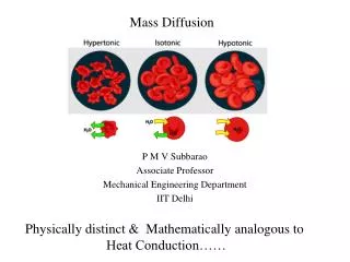
Diffusion Mass Transfer
DESCRIPTION
Diffusion Mass Transfer. Chapter 14 Sections 14.1 through 14.7. Lecture 18. Physical Origins and Rate Equations Mass Transfer in Nonstationary Media Conservation Equation and Diffusion through Stationary Media Diffusion and Concentrations at Interfaces
Download

1 / 0
Télécharger la présentation 
Diffusion Mass Transfer
An Image/Link below is provided (as is) to download presentation
Download Policy: Content on the Website is provided to you AS IS for your information and personal use and may not be sold / licensed / shared on other websites without getting consent from its author.
Content is provided to you AS IS for your information and personal use only.
Download presentation by click this link.
While downloading, if for some reason you are not able to download a presentation, the publisher may have deleted the file from their server.
During download, if you can't get a presentation, the file might be deleted by the publisher.
E N D
Presentation Transcript
-
Diffusion Mass Transfer
Chapter 14 Sections 14.1 through 14.7 Lecture 18 - Physical Origins and Rate Equations Mass Transfer in Nonstationary Media Conservation Equation and Diffusion through Stationary Media Diffusion and Concentrations at Interfaces Diffusion with Homogenous Reactions Transient Diffusion
- 1. Physical Origins and Rate Equations Driving potential for mass transfer Concentration Gradient Modes of mass transfer Convection and Diffusion
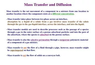
- General Considerations Mass transfer refers to mass in transit due to a species concentration gradient in a mixture. Must have a mixture of two or more species for mass transfer to occur. The species concentration gradient is the driving potential for transfer. Mass transfer by diffusion is analogous to heat transfer by conduction. Physical Origins of Diffusion: Transfer is due to random molecular motion. Consider two species A and B at the same T and p, but initially separated by a partition. Diffusion in the direction of decreasing concentration dictates net transport of A molecules to the right and B molecules to the left. In time, uniform concentrations of A and B are achieved.
- Definitions Molar concentration of species i. Mass density (kg/m3) of species i. Molecular weight (kg/kmol) of species i. Molar flux of species i due to diffusion. Absolute molar flux of species i. Mass flux of species i due to diffusion. Absolute mass flux of species i. Mole fraction of species i Mass fraction of species i Definitions Transport of i relative to molar average velocity (v*) of mixture. Transport of i relative to a fixed reference frame. Transport of i relative to mass-average velocity (v) of mixture. Transport of i relative to a fixed reference frame.
- Mixture Composition Definitions: Mass density of species i: i=Mi*Ci(kg/m3) Molecular weight of species i: Mi (kg/kmol) Molar concentration of species i: Ci (kmol/m3) Mixture mass density: (kg/m3) Total number of moles per unit volume of mixture
- Mixture Composition Definitions: Mass fraction of species i: mi=i/ Molar fraction of species i: xi=Ci/C For ideal gases:
- Fick’s Law of Diffusion For transfer of species A in a binary mixture of A & B Mass flux of species A (kg/m2s): Molar flux of species A (mol/m2s): Binary diffusivity DAB (m2/s) Ordinary diffusion due to concentration gradient and relative to coordinates that move with average velocity
- Fick’s Law of Diffusion For transfer of species A in a binary mixture of A & B Mass flux of species A (kg/m2s): Molar flux of species A (mol/m2s): If C and are constants, the above equations become:
- Mass Diffusivity For ideal gases At 298 K, 1 atm
- Example 14.1 Consider the diffusion of hydrogen (species A) in air, liquid water, or iron (species B) at T = 293 K. Calculate the species flux on both molar and mass bases if the concentration gradient at a particular location is dCA/dx= 1 kmol/m3●m. Compare the value of the mass diffusivity to the thermal diffusivity. The mole fraction of the hydrogen xA, is much less than unity.
- Example 14.1 Known:Concentration gradient of hydrogen in air, liquid water, or iron at 293 K Find: Molar and mass fluxes of hydrogen and the relative values of the mass diffusivity and thermal diffusivity Schematic:
- Example 14.1 Assumptions:Steady-state conditions Properties: Table A.8, hydrogen-air (298 K): DAB= 0.41x10⁻⁴ m2/s, hydrogen-water (298 K): DAB= 0.63x10⁻⁸ m2/s, hydrogen-iron (293 K): DAB= 0.26x10⁻¹² m2/s. Table A.4, air (293 K): α= 21.6x10⁻⁶ m2/s; Table A.6, water (293 K): k = 0.603 W/m•K, ρ = 998 kg/m3, cp= 4182 J/kg K. Table A.l, iron (300 K): α = 23.1 x 10⁻⁶m2/s. Analysis:Using Eqn. 14.14, we can find that the mass diffusivity of hydrogen in air at T=293K is
- Example 14.1 For the case where hydrogen is a dilute species, that is xA<<1, the thermal properties of the medium can be taken to be those of the host medium consisting of species B. The thermal diffusivity of water is: The ratio of the thermal diffusivity to the mass diffusivity is the Lewis number Le, defined in Equation 6.50. The molar flux of hydrogen is described by Fick’s law, Equation 14.13.
- Example 14.1 Hence, for the hydrogen-air mixture, The mass flux of hydrogen in air is found to from the expression:
- Example 14.1 The results for the three different mixtures are summarized in the following table:
- Mass Transfer in Nonstationary Media Absolute Mass Flux For mass flux relative to a fixed coordinate system Mass flux of species A (kg/m2s): Mass flux of species B (kg/m2s): Mass flux of mixture (kg/m2s): Mass-average velocity (m/s):
- Relative Mass Flux Mass flux of species A (kg/m2s): Mass flux of species A (kg/m2s):
- Relative Mass Flux Mass flux of species A (kg/m2s): Mass flux of species A (kg/m2s): For binary mixture of A & B:
- Relative Mass Flux For binary mixture of A & B: DAB=DBA
- Absolute Molar Flux For molar flux relative to a fixed coordinate system Molar flux of species A (mol/m2s): Mass flux of species B (kg/m2s): Mass flux of mixture (kg/m2s): Molar-average velocity (m/s):
- Absolute Molar Flux Molar flux of species A (kg/m2s): Mass flux of species A (kg/m2s):
- Absolute Molar Flux Mass flux of species B (kg/m2s): Mass flux of species B (kg/m2s): For binary mixture of A & B:
- Example 2 Gaseous H2 is stored at elevated pressure in a rectangular container having steel walls 10mm thick. The molar concentration of H2 in the steel at the inner surface is 1 kmol/m3, while the concentration of H2 in the steel at outer surface is negligible. The binary diffusion coefficient for H2 in steel is 0.26x10⁻¹² m2/s. what is the molar and mass diffusive flux for H2 through the steel?
- Example 2 Known:Molar concentration of H2 at inner and outer surfaces of a steel wall. Find: H2 molar and mass flux Schematic:
- Example 2 Assumptions: Steady-state, 1-D mass transfer conditions CA<<CB (H2 concentration much less than steel), total concentration C=CA+CB is uniform No chemical reaction between H2 and steel Analysis:
- Example 2 Analysis: (1). Simplify the molar flux equation
- Example 2 Analysis: (1). Simplify the molar flux equation 0
- Example 2 Analysis: (2). Apply C = constant
- Example 2 Analysis: (3). From mass conservation:
- Example 2 Analysis: (4). Integration from x=0 to x=L, CA=CA,1 to CA,2
- Example 2 Analysis: (5). Mass flux
- Evaporation in a Column
- Evaporation in a Column Assumptions: Ideal gases; No reaction; xA,0>xA,L, xB,0<xB,L; Gas B insoluble in liquid A
- Evaporation in a Column Stationary or moving medium?
- Evaporation in a Column Separate variables and integrate
- Evaporation in a Column Apply B.C.’s to solve C1 & C2:
- Example 3 An 8-cm-internal-diameter, 30-cm-high pitcher half Filled with water is left in a dry room at 15°C and 87 kPa with its top open. If the water is maintained at 15°C at all times also, determine how long it will take for the water to evaporate completely.
- Example 3
- Example 3
- Example 3 Lecture 18


More Related