SOLUTION FOR THE BOUNDARY LAYER ON A FLAT PLATE
320 likes | 907 Vues
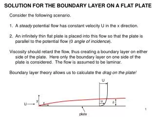
SOLUTION FOR THE BOUNDARY LAYER ON A FLAT PLATE. Consider the following scenario. A steady potential flow has constant velocity U in the x direction. An infinitely thin flat plate is placed into this flow so that the plate is parallel to the potential flow (0 angle of incidence ).

SOLUTION FOR THE BOUNDARY LAYER ON A FLAT PLATE
E N D
Presentation Transcript
SOLUTION FOR THE BOUNDARY LAYER ON A FLAT PLATE • Consider the following scenario. • A steady potential flow has constant velocity U in the x direction. • An infinitely thin flat plate is placed into this flow so that the plate is parallel to the potential flow (0 angle of incidence). • Viscosity should retard the flow, thus creating a boundary layer on either side of the plate. Here only the boundary layer on one side of the plate is considered. The flow is assumed to be laminar. • Boundary layer theory allows us to calculate the drag on the plate!
A STEADY RECTILINEAR POTENTIAL FLOW HAS ZERO PRESSURE GRADIENT EVERYWHERE A steady, rectilinear potential flow in the x direction is described by the relations According to Bernoulli’s equation for potential flows, the dynamic pressure of the potential flow ppd is related to the velocity field as Between the above two equations, then, for this flow
BOUNDARY LAYER EQUATIONS FOR A FLAT PLATE For the case of a steady, laminar boundary layer on a flat plate at 0 angle of incidence, with vanishing imposed pressure gradient, the boundary layer equations and boundary conditions become (see Slide 15 of BoundaryLayerApprox.ppt with dppds/dx = 0) Tangential and normal velocities vanish at boundary: tangential velocity = free stream velocity far from plate
NOMINAL BOUNDARY LAYER THICKNESS Until now we have not given a precise definition for boundary layer thickness. Here we use to denote nominal boundary thickness, which is defined to be the value of y at which u = 0.99 U, i.e. The choice 0.99 is arbitrary; we could have chosen 0.98 or 0.995 or whatever we find reasonable.
STREAMWISE VARIATION OF BOUNDARY LAYER THICKNESS Consider a plate of length L. Based on the estimate of Slide 11 of BoundaryLayerApprox.ppt, we can estimate as or thus where C is a constant. By the same arguments, the nominal boundary thickness up to any point x L on the plate should be given as
SIMILARITY One triangle is similar to another triangle if it can be mapped onto the other triangle by means of a uniform stretching. The red triangles are similar to the blue triangle. The red triangles are not similar to the blue triangle. Perhaps the same idea can be applied to the solution of our problem:
SIMILARITY SOLUTION Suppose the solution has the property that when u/U is plotted against y/ (where (x) is the previously-defined nominal boundary layer thickness) a universal function is obtained, with no further dependence on x. Such a solution is called a similarity solution. To see why, consider the sketches below. Note that by definition u/U = 0 at y/ = 0 and u/U = 0.99 at y/ = 1, no matter what the value of x. Similarity is satisfied if a plot of u/U versus y/ defines exactly the same function regardless of the value of x. Similarity satisfied Similarity not satisfied
SIMILARITY SOLUTION contd. So for a solution obeying similarity in the velocity profile we must have where g1 is a universal function, independent of x (position along the plate). Since we have reason to believe that where C is a constant (Slide 5), we can rewrite any such similarity form as Note that is a dimensionless variable. If you are wondering about the constant C, note the following. If y is a function of x alone, e.g. y = f1(x) = x2 + ex, then y is a function of p = 3x alone, i.e. y = f(p) = (p/3)2 + e(p/3).
BUT DOES THE PROBLEM ADMIT A SIMILARITY SOLUTION? Maybe, maybe not, you never know until you try. The problem is: This problem can be reduced with the streamfunction (u = /y, v = - /x) to: Note that the stream function satisfies continuity identically. We are not using a potential function here because boundary layer flows are not potential flows.
SOLUTION BY THE METHOD OF GUESSING We want our streamfunction to give us a velocity u = /y satisfying the similarity form So we could start off by guessing where f is another similarity function. But this does not work. Using the prime to denote ordinary differentiation with respect to , if = f() then But so that
SOLUTION BY THE METHOD OF GUESSING contd. So if we assume then we obtain This form does not satisfy the condition that u/U should be a function of alone. If F is a function of alone then its first derivative F’() is also a function of alone, but note the extra (and unwanted) functionality in x via the term (Ux)-1/2! So our first try failed because of the term (Ux)-1/2. Let’s not give up! Instead, let’s learn from our mistakes! not OK OK
ANOTHER TRY This time we assume Now remembering that x and y are independent of each other and recalling the evaluation of /y of Slide 10, or thus Thus we have found a form of that satisfies similarity in velocity! But this does not mean that we are done. We have to solve for the function F().
REDUCTION FROM PARTIAL TO ORDINARY DIFFERENTIAL EQUATION Our goal is to reduce the partial differential equation for and boundary conditions on , i.e. to an ordinary differential equation for and boundary conditions on f(), where To do this we will need the following forms:
REDUCTION contd. The next steps involve a lot of hard number crunching. To evaluate the terms in the equation below, we need to know /y, 2/y2, 3/y3, /x and 2/yx, where Now we have already worked out /y; from Slide 12: Thus
REDUCTION contd. Again using we now work out the two remaining derivatives:
REDUCTION contd. Summarizing,
REDUCTION contd. Now substituting into yields or thus Similarity works! It has cleaned up the mess into a simple (albeit nonlinear) ordinary differential equation!
BOUNDARY CONDITIONS From Slide 9, the boundary conditions are But we already showed that Now noting that = 0 when y = 0, the boundary conditions reduce to Thus we have three boundary conditions for the 3rd-order differential equation
SOLUTION There are a number of ways in which the problem can be solved. It is beyond the scope of this course to illustrate numerical methods for doing this. A plot of the solution is given below.
SOLUTION contd. To access the numbers, double-click on the Excel spreadsheet below. Recall that By interpolating on the table, it is seen that u/U = F’ = 0.99 when = 4.91.
NOMINAL BOUNDARY LAYER THICKNESS Recall that the nominal boundary thickness is defined such that u = 0.99 U when y = . Since u = 0.99 U when = 4.91 and = y[U/(x)]1/2, it follows that the relation for nominal boundary layer thickness is Or In this way the constant C of Slide 5 is evaluated.
DRAG FORCE ON THE FLAT PLATE Let the flat plate have length L and width b out of the page: The shear stress o (drag force per unit area) acting on one side of the plate is given as Since the flow is assumed to be uniform out of the page, the total drag force FD acting on (one side of) the plate is given as The term u/y = 2/y2 is given from (the top of) Slide 17 as b L
DRAG FORCE ON THE FLAT PLATE contd. The shear stress o(x) on the flat plate is then given as But from the table of Slide 20, f’’(0) = 0.332, so that boundary shear stress is given as Thus the boundary shear stress varies as x-1/2. A sample case is illustrated on the next slide for the case U = 10 m/s, = 1x10⁻⁶ m2/s, L = 10 m and = 1000 kg/m3 (water).
DRAG FORCE ON THE FLAT PLATE contd. Sample distribution of shear stress o(x) on a flat plate: U = 0.04 m/s L = 0.1 m = 1.5x10⁻⁵ m2/s = 1.2 kg/m3 (air) Note that o = at x = 0. Does this mean that the drag force FD is also infinite?
DRAG FORCE ON THE FLAT PLATE contd. No it does not: the drag force converges to a finite value! And here is our drag law for a flat plate! We can express this same relation in dimensionless terms. Defining a diimensionless drag coefficient cD as it follows that For the values of U, L, and of the last slide, and the value b = 0.05 m, it is found that ReL = 267, cD = 0.0407 and FD = 3.90x10⁻⁷ Pa.
DRAG FORCE ON THE FLAT PLATE contd. The relation is plotted below. Notice that the plot is carried only over the range 30 ReL 300. Within this range 1/ReL is sufficiently small to justify the boundary layer approximations. For ReL > about 300, however, the boundary layer is no longer laminar, and the effect of turbulence must be included.
REFERENCE The solution presented here is the Blasius-Prandtl solution for a boundary layer on a flat plate. More details can be found in: Schlichting, H., 1968, Boundary Layer Theory, McGraw Hill, New York, 748 p.