Download

1 / 101
1.01k likes | 1.15k Vues
This presentation covers essential concepts in computer vision, focusing on motion detection and stereo imaging. It introduces the geometry of motion and stereo analysis, including optical flow and motion estimation, to infer 3D information from 2D image sequences. Key techniques like background subtraction and disparity measurement will be discussed, along with the challenges of establishing correspondence in stereo images. The goal is to provide a foundational understanding of how motion and stereo imaging contribute to interpreting dynamic scenes in a 3D space.

E N D
Motion and Stereo EE4H, M.Sc 0407191 Computer Vision Dr. Mike Spann m.spann@bham.ac.uk http://www.eee.bham.ac.uk/spannm
Introduction • Computer vision involves the interpreting the time varying information on the 2D image plane in order to understand the position, shape and motion of objects in the 3D world • Through measurements of the optical flow, made using sequences of time varying images, or through measurements of disparity using a pair of images in a stereo image pair, we can infer 3D motion and position information from 2D images
Introduction • The topics we will consider are • The geometry of stereo and motion analysis • Motion detection • Background subtraction • Motion estimation • Optical flow • 3D motion and structure determination from image sequences • I will not cover feature point matching for stereo disparity determination as time is limited and motion analysis has more application
The geometry of motion and stereo • Consider a point P with co-ordinates (X,Y,Z) relative to a camera-centred co-ordinate system • The Z axis is oriented so that the axis points along the camera optical axis • Point P projects to point p(x,y) in the image plane
The geometry of motion and stereo • The projected coordinates on the image plane (x,y) are defined in terms of the perspective projection equation • f is the camera focal length
The geometry of motion and stereo • Suppose point P is moving with some velocity V • This projects to a velocity v on the image plane • This projected velocity is sometimes known as the optical flow
The geometry of motion and stereo • Optical flow is measurable from a set of frames of a video sequence • Using optical flow vectors measured at a large number of image locations, we can infer information about the 3D motion and object shape • Requires assumptions about the underlying 3D motion and surface shape
The geometry of motion and stereo • In the case of stereo imaging, we assume 2 cameras separated by some distance b • The measurement of disparity allows us to infer depth • The distance along the camera viewing axis
The geometry of motion and stereo • The disparity is the difference between the projected co-ordinates in the left and right stereo imagesxL- xR • Gives a measure of the depth • The greater the disparity, the lower the depth • The key task of stereo imaging is to establish a correspondence between image locations in the left and right camera image of an object point • This allows the depth of the imaged point to be computed either using the disparity or through triangulation
The geometry of motion and stereo • Triangulation enables the depth of an object point to be found given its image point in each camera
The geometry of motion and stereo • The geometry of stereo imaging is based on the epipolar constraint and the epipolar plane C C’
The geometry of motion and stereo • The epipolar line limits the search for a corresponding image point to one dimension • If the camera calibration parameters are known (intrinsic and extrinsic), the epipolar line for an image point in one camera can be computed
Motion detection/estimation • Motion detection aims to highlight areas of motion in an image • Motion areas can be defined by a binary ‘motion mask’
Motion detection/estimation • Motion estimation • Assigns a motion vector v(x,y)to each image pixel • Optical flow
Motion detection • Let the current frame be f (x, y, t) • Let f r(x, y, t) be a reference frame • d(x , y, t) highlights regions of large change relative to the reference frame • Normal to threshold d(x , y, t) to produce a binary motion mask m(x, y, t) and suppress noise
Motion detection • 2 usual cases • Frame differencing • Simple implementation but prone to noise and artefacts • Background subtraction • b(x, y, t) estimate of the (stationary) background at time t • More complex but yields a ‘cleaner’ motion mask
Motion detection • Fame differencing • Simple concept • Produces artefacts • Covered (occluded) and uncovered (disoccluded) regions highlighted whose size depends on the speed of the object relative to the video sampling rate • Very susceptible to inter-frame noise and illumination changes
Motion detection • Background subtraction • A ‘background’ image b(x ,y ,t) is computed which (hopefully!) is the stationary image over which objects move • The most simplistic approach is to average a number of previous frames • Or slightly more robust is to compute a weighted average
Motion detection • Both approaches lead to a background image that contain moving (foreground) objects • A better approach is to use a median filter • If the moving object is small enough such that it doesn’t overlap pixel (x,y) for more than T/2 frames it won’t appear in the background image • But, more susceptible to noise as it is not averaged out
Motion detection • Practical requirements: • The difference image is subtracted to compute a binary motion mask • Post thresholding enhancement • Morphological closing and opening to remove artefacts • Opening removes small objects, while closing removes small holes • Closing (I) = Erode(Dilate(I)) • Opening (I) = Dilate(Erode(I))
Motion detection • For improved performance in scenes that contain noise, illumination change and shadow effects more sophisticated methods are required • Statistical modelling of the background image • Simple greylevel intensity thresholds • W4 system • Gaussian models • Single Gaussian • Gaussian mixture models (GMM’s)
Motion detection • W4 system • Uses a training sequence containing only background (no moving objects) • Determine minimum Min(x,y)and maximum Max(x,y) intensity of background pixels • Determine the maximum difference between consecutive frames D(x, y) • Thresholding – f (x,y,t) foreground pixel if:
Motion detection • Complete W4 system is as follows: Background sequence Training Min(x,y), Max(x,y),D(x,y) Thresholding f(x,y,t) fb(x,y,t) Small region elimination Component analysis Opening,Closing
Motion detection • Gaussian models • Scalar grey-level or vector colour pixels • Single Gaussian model statistically models either the greyscale or colour of background pixels using a Gaussian distribution • Each background pixel (x,y) has its own Gaussian model represented by a mean µ(x,y) and standard deviation σ(x,y) for the case of greyscale images • For colour these become vectors and 3x3 matrices • For each frame, the mean and standard deviation images can be updated
Motion detection • Mean/standard deviation update • A simple foreground/background classification based on a log-likelihood function L(x, y, t)
Motion detection • Threshold t determines whether a pixel is a background pixel • The size of the threshold is a trade-off between false negative and false positive background pixels • Essentially the same as a background filter (with the background image being the mean and the threshold depending on the standard deviation)
Motion detection • Gaussian Mixture Model (GMM) • Scalar greylevel or vector colour pixels • A single Gaussian distribution cannot characterize an image with: • Noise • None uniform illumination • Complex scene content • Variation in light illumination • A GMM has been shown to represent more faithfully the variation in greylevel or colour at each background pixel
Motion detection • The GMM models the probability distribution of each pixel as a mixture of N (typically 3) Gaussian distributions
Motion detection • Mixture model dynamically updated • If a pixel f(x,y,t) within 2.5 standard deviations of the kthmode, the parameters of that mode are updated:
Motion detection • Detection of Foreground / Background • Compute w/s for each distribution • Sort in descending order of w/s • First B Gaussian modes represent the background:
Motion detection • The final method combines a simple frame differencing method with relaxation labelling to reduce noise • Use pforeground for neighbouring pixels in space to update the probabilities and exploit the spatial continuity of moving objects • Doesn’t have the problem of ‘ghosting’ that background subtraction has • Can implement the simple iterative relaxation labelling algorithm efficiently for close to normal frame rate performance
Motion detection • Demo
Motion estimation – Optical flow • Background subtraction algorithms detect motion but don’t give us an estimate of the motion • Many applications in 3D vision require an estimate of the motion (pixels/second) – see later! • Also background subtraction algorithms require a static background • More difficult (but not impossible) when the camera is moving • The main difficulty with optical flow is computing it robustly!
Motion estimation – Optical flow • Optical flow is a pixel-wise estimate of the motion • It relates to the real 3D velocities which are projected onto the image plane • A displacement V(X,Y,Z )t in 3Dprojects to a displacement v(x,y) t in the image plane • v(x,y) t is called the displacement • v(x,y) is called the optical flow • 2 approaches to computing flow • Feature matching • Gradient based methods
Computing optical flow • Feature matching involves matching some small image region between successive frames in an image sequence or between stereo pairs • Leads to a sparse flow field v(x,y) • Usually involves matching corner points or other ‘interesting’ regions • Involves detecting suitable features and assigning correct correspondences
Computing optical flow Left Right
Computing optical flow • In gradient-based methods, the greylevel profile is assumed to be locally linear which can be matched in the image pair • The implied assumption is that the local displacement between images is small • This is the normal approach to the estimation of a dense optical flow field in image sequences
Computing optical flow • Gradient-based methods assume a linear-ramped greylevel edge is displaced by vt between 2 successive frame • Easy to relate the change in greylevel to the gradient and optical flow v • We will look in detail at an algorithm later
Computing optical flow vt v t t+t x x+x
Computing optical flow • We can derive a simple expression for optical flow by considering a 1D greylevel ramp moving with a speed of in the x direction
Computing optical flow Gradient of ramp = Greylevel conservation equation
Computing optical flow • In 2D we have a planar surface translating with velocity (vx,vy) Greylevel gradient vector
Computing optical flow • In 2D, the greylevel conservation equation becomes : • Or in vector notation
Computing optical flow • We can explicitly derive the 2D conservation equation by considering a 2D greylevel patch moving with velocity v= (vx,vy)