High Dynamic Range Images
High Dynamic Range Images. cs195g: Computational Photography James Hays, Brown, Spring 2010. slides from Alexei A. Efros and Paul Debevec. Problem: Dynamic Range. 1. The real world is high dynamic range. 1500. 25,000. 400,000. 2,000,000,000. Long Exposure. 10 -6. 10 6.


High Dynamic Range Images
E N D
Presentation Transcript
High Dynamic Range Images cs195g: Computational Photography James Hays, Brown, Spring 2010 slides from Alexei A. Efrosand Paul Debevec
Problem: Dynamic Range 1 The real world ishigh dynamic range. 1500 25,000 400,000 2,000,000,000
Long Exposure 10-6 106 High dynamic range Real world 10-6 106 Picture 0 to 255
Short Exposure 10-6 106 High dynamic range Real world 10-6 106 Picture 0 to 255
Image pixel (312,284) = 42 42 photons?
Camera Calibration • Geometric • How pixel coordinatesrelate todirectionsin the world • Photometric • How pixel valuesrelate toradianceamounts in the world
Camera Calibration • Geometric • How pixel coordinatesrelate todirectionsin the world in other images. • Photometric • How pixel valuesrelate toradianceamounts in the world in other images.
ò The ImageAcquisition Pipeline Lens Shutter scene radiance (W/sr/m ) sensor irradiance sensor exposure 2 Dt CCD ADC Remapping analog voltages digital values pixel values Raw Image JPEGImage
Imaging system response function 255 Pixel value 0 log Exposure = log (Radiance * Dt) (CCD photon count)
Camera is not a photometer! • Limited dynamic range • Perhaps use multiple exposures? • Unknown, nonlinear response • Not possible to convert pixel values to radiance • Solution: • Recover response curve from multiple exposures, then reconstruct the radiance map
Recovering High Dynamic RangeRadiance Maps from Photographs Paul Debevec Jitendra Malik Computer Science Division University of California at Berkeley August 1997
Ways to vary exposure • Shutter Speed (*) • F/stop (aperture, iris) • Neutral Density (ND) Filters
Shutter Speed • Ranges: Canon D30: 30 to 1/4,000 sec. • Sony VX2000: ¼ to 1/10,000 sec. • Pros: • Directly varies the exposure • Usually accurate and repeatable • Issues: • Noise in long exposures
Shutter Speed • Note: shutter times usually obey a power series – each “stop” is a factor of 2 • ¼, 1/8, 1/15, 1/30, 1/60, 1/125, 1/250, 1/500, 1/1000 sec • Usually really is: • ¼, 1/8, 1/16, 1/32, 1/64, 1/128, 1/256, 1/512, 1/1024 sec
The Algorithm Image series • 1 • 1 • 1 • 1 • 1 • 2 • 2 • 2 • 2 • 2 • 3 • 3 • 3 • 3 • 3 Dt =1/64 sec Dt =1/16 sec Dt =1/4 sec Dt =1 sec Dt =4 sec Pixel Value Z = f(Exposure) Exposure = Radiance *Dt log Exposure =log Radiance + log Dt
Assuming unit radiance for each pixel After adjusting radiances to obtain a smooth response curve 3 2 Pixel value Pixel value Response Curve 1 ln Exposure ln Exposure
The Math • Let g(z) be the discrete inverse response function • For each pixel site i in each image j, want: • Solve the overdetermined linear system: fitting term smoothness term
function [g,lE]=gsolve(Z,B,l,w) n = 256; A = zeros(size(Z,1)*size(Z,2)+n+1,n+size(Z,1)); b = zeros(size(A,1),1); k = 1; %% Include the data-fitting equations for i=1:size(Z,1) for j=1:size(Z,2) wij = w(Z(i,j)+1); A(k,Z(i,j)+1) = wij; A(k,n+i) = -wij; b(k,1) = wij * B(i,j); k=k+1; end end A(k,129) = 1; %% Fix the curve by setting its middle value to 0 k=k+1; for i=1:n-2 %% Include the smoothness equations A(k,i)=l*w(i+1); A(k,i+1)=-2*l*w(i+1); A(k,i+2)=l*w(i+1); k=k+1; end x = A\b; %% Solve the system using SVD g = x(1:n); lE = x(n+1:size(x,1)); MatlabCode
Results: Digital Camera Kodak DCS4601/30 to 30 sec Recovered response curve Pixel value log Exposure
Results: Color Film • Kodak Gold ASA 100, PhotoCD
Recovered Response Curves Red Green Blue RGB
Portable FloatMap (.pfm) • 12 bytes per pixel, 4 for each channel sign exponent mantissa Text header similar to Jeff Poskanzer’s .ppmimage format: PF 768 512 1 <binary image data> Floating Point TIFF similar
Radiance Format(.pic, .hdr) 32 bits / pixel Red Green Blue Exponent (145, 215, 87, 103) = (145, 215, 87) * 2^(103-128) = (0.00000432, 0.00000641, 0.00000259) (145, 215, 87, 149) = (145, 215, 87) * 2^(149-128) = (1190000, 1760000, 713000) Ward, Greg. "Real Pixels," in Graphics Gems IV, edited by James Arvo, Academic Press, 1994
ILM’s OpenEXR (.exr) • 6 bytes per pixel, 2 for each channel, compressed sign exponent mantissa • Several lossless compression options, 2:1 typical • Compatible with the “half” datatype in NVidia's Cg • Supported natively on GeForce FX and Quadro FX • Available athttp://www.openexr.net/
Tone Mapping • How can we do this? Linear scaling?, thresholding? Suggestions? 10-6 106 High dynamic range Real World Ray Traced World (Radiance) 10-6 106 Display/ Printer 0 to 255
TheRadianceMap Linearly scaled to display device
Simple Global Operator • Compression curve needs to • Bring everything within range • Leave dark areas alone • In other words • Asymptote at 255 • Derivative of 1 at 0
Darkest 0.1% scaled to display device Reinhart Operator
What do we see? Vs.
Issues with multi-exposure HDR • Scene and camera need to be static • Camera sensors are getting better and better • Display devices are fairly limited anyway (although getting better).