Download
1 / 27
270 likes | 293 Vues
Explore power spectra characteristics and theoretical background of stellar oscillations, including radial and non-radial modes, with propagation diagrams and observed parameters. Predict power spectra based on basic assumptions.

E N D
Theoretical Interpretation of Power Spectra of Stellar Oscillations • H.Ando • National Astronomical Observatory of Japan • 9th, December, 2004
1. Observed Power Spectra of Stellar Oscillations Procyon(F5 subg) Kambe (2000) Sun, αCen A, βHyi(G2 subg), η Boo(G0 subg), ξ Hya(G7 g) Bedding and Kjeldsen (2003) PASA, 20, 203-212
Summed spectrum of Procyon on 25, 28, and 29, Dec., 2000
Charactristics of Spectra ・shape of envelope (peak freq.) ・Asymptotic Formula Large separation Small Separation
Newly recognized points ・Not a simple distribution of amplitudes ・Deviation from equal spacing pattern
2. Theoretical background of Oscillations ・Radial Pulsation (l=0) acoustic modes(n=0,1,2,....) fn(r) ・non-radial oscillation(l≠0) acoustic modes (p-mode) (n,l,m) gravity modes (g-mode)(n,l,m) fn(r)Ylm(θ,φ)
Propagation diagram in Stars ex. Procyon M=1.42 M⦿ (Prieto et. al 2002) #1(ZAMS) #51 (Procyon; L=7L⦿, Te=6530) #211(giant; L=7.7L⦿, Te=4490) Observed parameters of Procyon L= 7.04L⦿ , Te= 6530
Propagation diagram for #1 36 36 0 2236.61 47.29 5.90E-07 35 35 0 2116.27 46.00 8.05E-07 34 34 0 1999.02 44.71 9.92E-07 33 33 0 1884.98 43.42 1.15E-06 32 32 0 1774.07 42.12 1.29E-06 31 31 0 1666.27 40.82 1.40E-06 30 30 0 1561.78 39.52 1.48E-06 29 29 0 1460.84 38.22 1.53E-06 28 28 0 1363.62 36.93 1.55E-06 27 27 0 1270.12 35.64 1.54E-06 26 26 0 1180.19 34.35 1.52E-06 25 25 0 1093.67 33.07 1.49E-06 24 24 0 1010.51 31.79 1.45E-06 23 23 0 930.78 30.51 1.42E-06 22 22 0 854.58 29.23 1.40E-06 21 21 0 781.89 27.96 1.40E-06 20 20 0 712.57 26.69 1.42E-06 19 19 0 646.44 25.43 1.46E-06 18 18 0 583.36 24.15 1.49E-06 17 17 0 523.35 22.88 1.51E-06 16 16 0 466.58 21.60 1.52E-06 15 15 0 413.22 20.33 1.50E-06 14 14 0 363.33 19.06 1.47E-06 13 13 0 316.95 17.80 1.41E-06 12 12 0 274.08 16.56 1.33E-06 11 11 0 234.74 15.32 1.25E-06 10 10 0 198.94 14.10 1.19E-06 9 9 0 166.66 12.91 1.23E-06 8 8 0 137.71 11.73 1.42E-06 7 7 0 111.79 10.57 1.91E-06 6 6 0 88.70 9.42 2.97E-06 5 5 0 68.21 8.26 5.43E-06 4 4 0 50.49 7.11 1.14E-05 3 3 0 35.37 5.95 2.91E-05 2 2 0 22.92 4.79 1.02E-04 1 1 0 12.80 3.58 7.99E-04 -1 0 1 4.23 2.06 6.11E-01 -2 0 2 1.97 1.41 7.14E-01 P G P G
25 25 0 1224.07 34.99 3.05E-06 24 24 0 1131.91 33.64 3.21E-06 23 23 0 1043.65 32.31 3.38E-06 22 22 0 959.17 30.97 3.48E-06 21 21 0 879.00 29.65 3.59E-06 20 20 0 802.57 28.33 3.83E-06 19 19 0 746.14 27.32 1.42E-04 18 19 1 728.52 26.99 4.35E-06 17 18 1 659.75 25.69 4.33E-06 16 17 1 593.52 24.36 4.72E-06 15 16 1 530.53 23.03 5.13E-06 14 15 1 470.90 21.70 5.54E-06 13 14 1 414.70 20.36 5.86E-06 12 13 1 362.18 19.03 6.03E-06 11 12 1 319.80 17.88 9.31E-04 10 12 2 313.30 17.70 6.11E-06 9 11 2 268.43 16.38 5.81E-06 8 10 2 227.25 15.07 5.51E-06 7 9 2 189.91 13.78 5.02E-06 6 8 2 167.35 12.94 6.05E-03 5 8 3 156.58 12.51 4.58E-06 4 7 3 127.08 11.27 4.37E-06 3 6 3 105.14 10.25 1.12E-03 2 6 4 101.36 10.07 4.58E-06 1 5 4 79.28 8.90 5.75E-06 0 4 4 73.00 8.54 1.80E-03 -1 4 5 60.86 7.80 9.30E-06 -2 3 5 53.57 7.32 5.26E-04 -3 3 6 47.92 6.92 2.70E-05 -4 3 7 41.58 6.45 6.67E-05 -5 2 7 39.04 6.25 8.00E-05 -6 2 8 32.63 5.71 1.70E-04 -7 2 9 30.25 5.50 1.39E-04 -8 2 10 26.37 5.14 2.36E-04 -9 1 10 24.17 4.92 4.53E-04 P G P G
211 1 -23 22 45 1097.25 33.12 2.65E-05 -24 22 46 1060.79 32.57 6.50E-06 -25 21 46 1046.33 32.35 1.15E-05 -26 21 47 1009.25 31.77 1.01E-04 -27 21 48 975.16 31.23 1.78E-05 -28 21 49 962.36 31.02 1.82E-05 -29 20 49 930.81 30.51 2.01E-04 -30 20 50 897.73 29.96 8.23E-05 -31 20 51 882.12 29.70 1.95E-05 -32 19 51 860.46 29.33 2.05E-04 -33 19 52 830.45 28.82 3.23E-04 -34 19 53 806.29 28.40 3.59E-05 -35 19 54 795.75 28.21 6.40E-05 -36 18 54 770.81 27.76 5.44E-04 -37 18 55 745.08 27.30 4.06E-04 -38 18 56 726.23 26.95 4.20E-05 -39 17 56 716.05 26.76 1.23E-04 -40 17 57 694.02 26.34 8.00E-04 -41 17 58 671.87 25.92 6.44E-04 -42 17 59 653.85 25.57 7.07E-05 -43 17 60 645.80 25.41 9.67E-05 -44 16 60 627.81 25.06 8.81E-04 -45 16 61 608.60 24.67 1.22E-03 -46 16 62 590.72 24.30 3.20E-04 -47 16 63 580.86 24.10 6.02E-05 -48 15 63 570.18 23.88 4.37E-04 -49 15 64 553.83 23.53 1.64E-03 -50 15 65 537.77 23.19 1.58E-03 -51 15 66 522.89 22.87 3.66E-04 -52 15 67 514.61 22.68 7.27E-05 -53 14 67 505.59 22.49 4.93E-04 -54 14 68 491.91 22.18 1.96E-03 -55 14 69 478.35 21.87 2.31E-03 -56 14 70 465.50 21.58 9.38E-04 -57 14 71 455.57 21.34 1.08E-04 -58 14 72 450.26 21.22 1.92E-04 -59 13 72 439.52 20.96 1.54E-03 -60 13 73 428.07 20.69 3.16E-03 -61 13 74 417.01 20.42 2.85E-03 -62 13 75 406.54 20.16 1.09E-03 -63 13 76 398.22 19.96 1.27E-04 -64 13 77 393.84 19.85 1.89E-04 G P G P
Interaction bet ween Two potential wells ・ZAMS: Almost independent
・Advanced Evolution stage: Mixed character Avoided Crossing
Mixed Mode
3. Prediction of Power Spectra Basic assumptions ・Power ∝ (Input Energy)/(Kinetic Energy of mode), where KE is estimated with radial displacement, say(δr/r=1.0), at the surface. ・Input Energy Continuous spectrum by turbulent convection (Kolmogorov spectrum) We give Power ∝ f^n/(KE) n=2 : flat input energy (say, 1m/s at the surface) n=-2: Kolmogorov type input energy
Summary ・There are pulsation modes (l=0) beyond Cut-off frequency ・There are practical cut-off in lower end due to existence of g-modes’ territory ・Larger interaction of p-modes and g-modes in l=1 -modes with smaller amplitudes in mixed modes -frequencies of modes(l=1) shifted to modes with l=0 in lower frequency region
A possible suggestion Quantitative analysis of the Oscillation spectrum of ηBoo Guenther AJ, 612, 454-462, 2004